Differential celltype composition between groups
Sarah Williams (Author)
James Sinclair (User Review)
Laurelle Jackson (User Review)
Last updated: 2025-03-13
Checks: 7 0
Knit directory: spatialsnippets/
This reproducible R Markdown analysis was created with workflowr (version 1.7.1). The Checks tab describes the reproducibility checks that were applied when the results were created. The Past versions tab lists the development history.
Great! Since the R Markdown file has been committed to the Git repository, you know the exact version of the code that produced these results.
Great job! The global environment was empty. Objects defined in the global environment can affect the analysis in your R Markdown file in unknown ways. For reproduciblity it’s best to always run the code in an empty environment.
The command set.seed(20231017) was run prior to running
the code in the R Markdown file. Setting a seed ensures that any results
that rely on randomness, e.g. subsampling or permutations, are
reproducible.
Great job! Recording the operating system, R version, and package versions is critical for reproducibility.
Nice! There were no cached chunks for this analysis, so you can be confident that you successfully produced the results during this run.
Great job! Using relative paths to the files within your workflowr project makes it easier to run your code on other machines.
Great! You are using Git for version control. Tracking code development and connecting the code version to the results is critical for reproducibility.
The results in this page were generated with repository version 4992673. See the Past versions tab to see a history of the changes made to the R Markdown and HTML files.
Note that you need to be careful to ensure that all relevant files for
the analysis have been committed to Git prior to generating the results
(you can use wflow_publish or
wflow_git_commit). workflowr only checks the R Markdown
file, but you know if there are other scripts or data files that it
depends on. Below is the status of the Git repository when the results
were generated:
Ignored files:
    Ignored:    .Rhistory
    Ignored:    .Rproj.user/
    Ignored:    analysis/contributions.nb.html
    Ignored:    analysis/d_cosmxIBD_sfe.nb.html
    Ignored:    analysis/d_test.nb.html
    Ignored:    analysis/e_neighbourcellchanges.nb.html
    Ignored:    analysis/e_spatiallyRestrictedGenesVoyager.nb.html
    Ignored:    analysis/g_toolkits.nb.html
    Ignored:    analysis/glossary.nb.html
    Ignored:    renv/library/
    Ignored:    renv/staging/

Untracked files:
    Untracked:  code/scwat-at_betweenClusters_heterotypic_score_functions.R
    Untracked:  other/

Unstaged changes:
    Modified:   analysis/d_cosmxIBD_sfe.Rmd
    Modified:   renv.lock
    Modified:   renv/activate.R
    Modified:   spatialsnippets.Rproj
Note that any generated files, e.g. HTML, png, CSS, etc., are not included in this status report because it is ok for generated content to have uncommitted changes.
These are the previous versions of the repository in which changes were
made to the R Markdown (analysis/e_CompositionChange.Rmd)
and HTML (docs/e_CompositionChange.html) files. If you’ve
configured a remote Git repository (see ?wflow_git_remote),
click on the hyperlinks in the table below to view the files as they
were in that past version.
| File | Version | Author | Date | Message |
|---|---|---|---|---|
| Rmd | 4992673 | swbioinf | 2025-03-13 | wflow_publish("analysis/e_CompositionChange.Rmd") |
| html | 9989fa8 | swbioinf | 2024-08-23 | Build site. |
| Rmd | 5cae056 | swbioinf | 2024-08-23 | wflow_publish(c("analysis/e_CompositionChange.Rmd")) |
| html | 53dff19 | swbioinf | 2024-08-23 | Build site. |
| Rmd | 46145cf | swbioinf | 2024-08-23 | wflow_publish(c("analysis/e_CompositionChange.Rmd")) |
| html | 4d21ff2 | swbioinf | 2024-05-31 | Build site. |
| Rmd | 29b171b | swbioinf | 2024-05-31 | wflow_publish("analysis/e_CompositionChange.Rmd") |
| html | a6dd41e | swbioinf | 2024-05-31 | Build site. |
| Rmd | 46429ac | swbioinf | 2024-05-31 | wflow_publish("analysis/e_CompositionChange.Rmd") |
| html | 6978154 | swbioinf | 2024-05-30 | Build site. |
| Rmd | f14901b | swbioinf | 2024-05-30 | wflow_publish(c("analysis/e_DEPseudobulk_insitu.Rmd", "analysis/e_CompositionChange.Rmd", |
| html | 0af0a41 | swbioinf | 2024-05-08 | Build site. |
| Rmd | 3b66014 | swbioinf | 2024-05-08 | wflow_publish(c("analysis/e_CompositionChange.Rmd")) |
| html | cfa2539 | swbioinf | 2024-05-07 | Build site. |
| Rmd | a258ba3 | swbioinf | 2024-05-07 | wflow_publish(c("analysis/e_CompositionChange.Rmd")) |
| html | 03a38b8 | swbioinf | 2024-05-07 | Build site. |
| Rmd | 469bf34 | swbioinf | 2024-05-07 | wflow_publish("analysis/e_CompositionChange.Rmd") |
| html | 3a1bdf3 | swbioinf | 2024-05-07 | Build site. |
| Rmd | 5e7e7fb | swbioinf | 2024-05-07 | wflow_publish("analysis/e_CompositionChange.Rmd") |
| html | 4eb5dd9 | swbioinf | 2024-05-03 | Build site. |
| Rmd | 49d07d2 | swbioinf | 2024-05-03 | wflow_publish("analysis/e_CompositionChange.Rmd") |
| html | 2441c2d | swbioinf | 2024-04-23 | Build site. |
| Rmd | 96fcd96 | swbioinf | 2024-04-23 | wflow_publish("analysis/e_CompositionChange.Rmd") |
| html | 22b7d61 | swbioinf | 2024-04-22 | Build site. |
| Rmd | 4701a50 | swbioinf | 2024-04-22 | wflow_publish("analysis/e_CompositionChange.Rmd") |
| html | a722f36 | swbioinf | 2024-04-18 | Build site. |
| Rmd | 1dc6730 | swbioinf | 2024-04-18 | wflow_publish(c("analysis/index.Rmd", "analysis/e_CompositionChange.Rmd", |
| html | 8423279 | swbioinf | 2024-04-17 | Build site. |
| Rmd | 048c672 | swbioinf | 2024-04-17 | wflow_publish("analysis/e_CompositionChange.Rmd") |
| html | 456dd2f | swbioinf | 2024-04-10 | Build site. |
| Rmd | 8ef9cd9 | swbioinf | 2024-04-10 | wflow_publish("analysis/") |
| html | 30da140 | Sarah Williams | 2024-03-22 | Build site. |
| Rmd | 89c3371 | Sarah Williams | 2024-03-22 | wflow_publish(c("analysis/index_data.Rmd", "analysis/index.Rmd", |
Overview
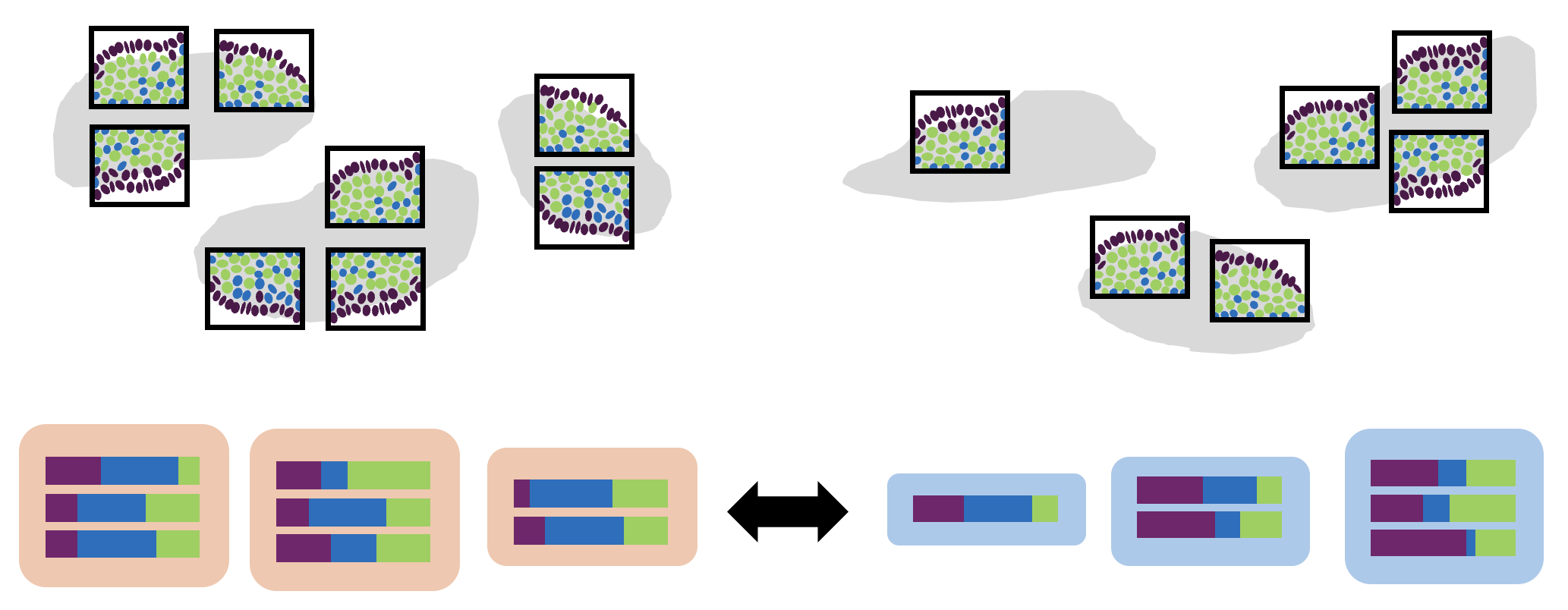
With single cell spatial data, the frequency of each cell type can be tested between two different groups.
Testing changes in proportions like this can be challenging, because an expansion in one cell type, will mean a reduction in all other cell types.
This document describes how to use the propeller (Phipson et al. 2022) method from the speckle R package, and limma to test for differences in cell type proportions. This takes into account this linked relationship between cell type proportions, and can incorporate pseudoreplicate data from multiple FOVs (fields of view) from an insitu single cell spatial dataset.
This requires:
- Biological replicates for each group
- Assigned cell types
- [Optionally] Multiple fovs measured per sample
For example:
- Are there more macrophages around the tumour after treatment?
- Is there a celltype that’s failing to form (or an immature form that’s failing to develop) between d3 and d7 in my mouse knockouts?
Worked example
This example uses the data from paper Macrophage and neutrophil heterogeneity at single-cell spatial resolution in human inflammatory bowel disease from Garrido-Trigo et al 2023, (Garrido-Trigo et al. 2023)
The study included 9 cosmx slides of colonic biopsies
- 3x HC - Healthy controls
- 3x UC - Ulcerative colitis
- 3x CD - Chrones’s disease
Is there a difference in the celltype composition between individuals with Ulcerative colitis or Crohn’s disease, and Healthy controls?
Load libraries and data
library(Seurat)
library(speckle)
library(tidyverse)
library(limma)
library(DT)
data_dir <- file.path("~/projects/spatialsnippets/datasets/GSE234713_IBDcosmx_GarridoTrigo2023/processed_data")
seurat_file_01_loaded <- file.path(data_dir, "GSE234713_CosMx_IBD_seurat_01_loaded.RDS")so <- readRDS(seurat_file_01_loaded)Experimental design
There are three individuals per condition (one tissue sample from each individual). With multiple fovs on each physical tissue sample.
sample_table <- select(as_tibble(so@meta.data), condition, individual_code, fov_name) %>%
  unique() %>%
  group_by(condition, individual_code) %>%
  summarise(n_fovs= n(), item = str_c(fov_name, collapse = ", "))

DT::datatable(sample_table)
Count how many cells of each type in your data
In this dataset there are actually two different levels of categorisation;
- Celltype_subset: Some broad groupings of cell types.
- celltype_SingleR2: Much more specific groupings, predicted with the singleR method (Aran et al. 2019)
Lets check the numbers of cells per category for both categories, to decide which we can use. We’d like to look at the celltype proportions at the most specific resolution - but we need to ensure there are enough cells of each type for meaningful statistics.
In the ‘Celltype_subset’ column, there are just 5 broad categories;
celltype_summary_table <- so@meta.data %>%
  group_by(condition, group, individual_code, fov_name, celltype_subset) %>%
  summarise(cells=n(), .groups = 'drop')
DT::datatable(celltype_summary_table)
There are many different types in ‘celltype_SingleR2’ - which is typical if you’re using celltype assignment with a detailed reference.
celltype_summary_table.SingleR <- so@meta.data %>%
  group_by(condition, group, individual_code, fov_name, celltype_SingleR2) %>%
  summarise(cells=n(), .groups = 'drop')
DT::datatable(celltype_summary_table.SingleR)
Check your celltype categories
For both categories, plot how many we see per FOV on average.
In the ‘celltype_subset’ category, T cells are rare, but there are still a decent distribution of them with 10-100+ cells in a FOV. We should be able to see changes in these.
ggplot(celltype_summary_table, aes(x=cells, col=celltype_subset)) +
  geom_density() +
  geom_rug(alpha=0.2) +
  scale_x_log10() +
  theme_bw() +
  ggtitle("Cells per FOV by celltype")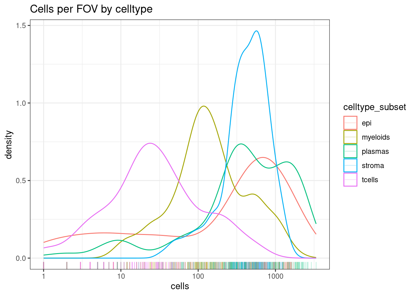
On the other hand, could we use the more fine-grained categorisation in the ‘celltype_SingleR2’ grouping?
In this case, there are just too many cell type categories, and we should stick with the broad categorisation.
ggplot(celltype_summary_table.SingleR, aes(x=cells, col=celltype_SingleR2)) +
  geom_density() +
  geom_rug(alpha=0.2) +
  scale_x_log10() +
  theme_bw() +
  ggtitle("Cells per FOV by celltype")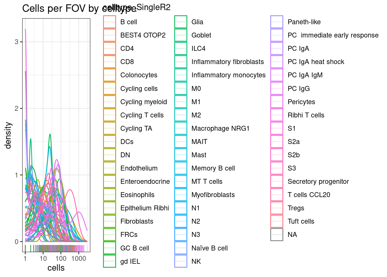
Approaches to make use of more specific groupings.
You might still want to use a more specific grouping. You might be able to tweak your groups to make this happen.
Some possible approaches:
- Drop ‘nonsense’ cell types: When cell typing with a broad reference, you might get a handful of irrelevant cell types called (e.g. 4 hepatocytes on a non-liver sample).
- Pool subtypes: Some celltypes are simply rare. Rather then dropping them entirely, you can pool transcriptionally similar cells (e.g. T cell subtypes).
The more cell types you have, the more aggressive your FDR multiple hypothesis correction will need to be. Its best to remove or condense cell types that can never reach statistical significance.
Look at your samples
In a RNAseq experiment, you would typically have one set of measurements per biological sample. In a single cell RNAseq experiment you’d typically have one group of cells measured for that same sample. With the current crop of spatially resolved single cell technologies (e.g. cosmx), you can have multiple FOVs (feilds of view) on the same physical chunk of tissue. These are not true biological replicates and can be considered ‘pseudoreplicates’.
Pseudoreplicates can still have a degree of heterogeneity, from different regions of the tissue. E.g. some samples might overlap epithelial regions more than others.
Lets plot the cell type composition across all the pseodureplicates, grouped by replicate, and grouped by condition. Where there are more samples or uneven numbers, it might be helpful to plot each condition separately.
ggplot(celltype_summary_table, aes(x=fov_name, y=cells, fill=celltype_subset)) +
  geom_bar(position="fill", stat="identity") +
  theme_bw() +
  coord_flip() +
  theme(legend.position = "bottom") +
  facet_wrap(~individual_code, ncol=3, scales = 'free_y')  +
scale_y_continuous(expand = c(0,0)) 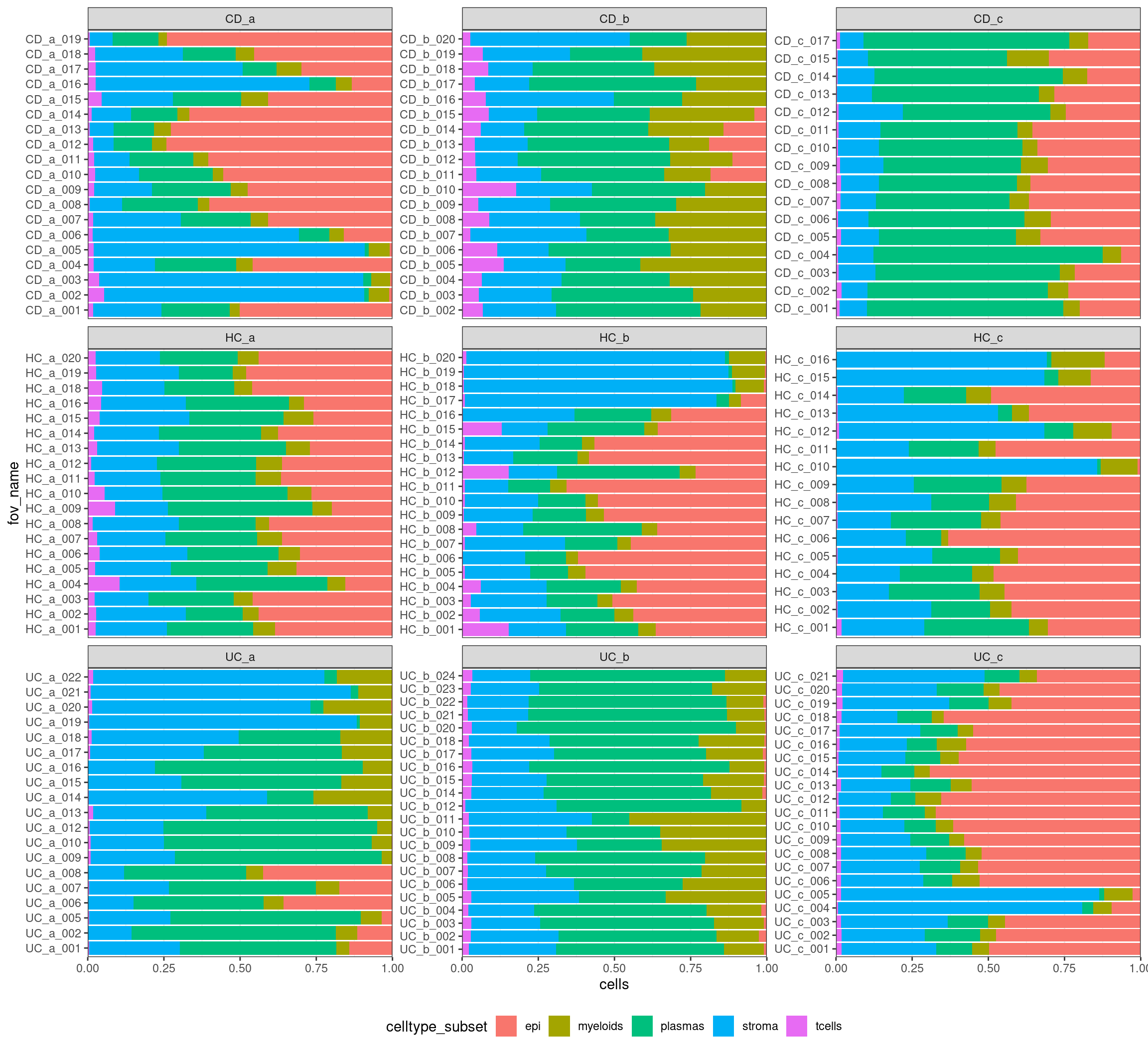
If there are obvious changes in cell type proportions, they should be visible now!
- Are there differences in the tissue regions targeted by the fovs? e.g. Epithealial vs stromal? Consider whether it is appropriate to include fovs together.
- Are you capturing regions or structures of different sizes that you don’t want to test? e.g. Fovs at the epithalial edge might have uninteresting differences in epthialial cells counts, just through fov placement choices. Omitting the epithelial cell counts might be appropriate to measure differences in the rest.
Calculate stats
Now we can formally test for differences.
For the simple case where there are no fov pseudoreplicats (e.g a
single cell RNAseq experiment), there is a propellar
function. This approach is described in the speckle
vignette
# Without FOV replicates - Not what we want.
results_table.no_fov_info <- propeller(clusters = so$celltype_subset,
                           sample   = so$individual_code,
                           group    = so$condition)
DT::datatable(results_table.no_fov_info)
It would be possible to counts cells at the sample level, and use the above method. But - having seen the within sample heterogeneity across multiple fovs, we want to take that into account. This takes few more steps, using the limma (Ritchie et al. 2015) duplicateCorrealation approach described in the speckle vignette here
Calculate the transformed proportion that speckle needs on each fov.
props <- getTransformedProps(so$celltype_subset, so$fov_name, transform="logit")Then use limma to test for differences.
If you are not familiar with limma, or you want more info on building your own ‘design’ or ‘contrasts’ there are many online resources that cover it. For example the substantial limma documentation, or online tutorials such as this one or any number of forum posts. The instructions for RNAseq or microarray differential expression tests can be applied to this proportional data. The difference is that we provide the proportions.
# The fovs as ordered in props
fov_name <- colnames(props$TransformedProps)

# Extract the other information in the same order.
# Note we're using the group column with simple names (entries like 'CD', 'HC') rather than the condition column ("Chron's Disease", "Healthy controls").
# This is because differential tests with limma doesn't handle spaces and special characters (like ',- ) very well at all.
props_order <- match(fov_name, celltype_summary_table$fov_name)
clusters <- celltype_summary_table$celltype_subset[props_order]
sample   <- celltype_summary_table$individual_code[props_order]
group    <- celltype_summary_table$group[props_order]

# Build the design matrix
# This simple one considers only the disease.
# and includes the 0+ term to avoid setting one group to our baseline, which in turn  make building contrasts more intuative.
design <- model.matrix( ~ 0+ group)

# Calculate duplicate correlation, within fovs for different individuals (sample)
dupcor <- duplicateCorrelation(props$TransformedProps, design=design,  block=sample)


# Next fit the model to your data; using the experimental design, blocking on the individual/sample, and providing the 'consensus' correlation value from duplicate correlation.
fit <- lmFit(props$TransformedProps, design=design, block=sample, correlation=dupcor$consensus)

# These are the groups from the model (not the prefixed 'group')
colnames(fit)
[1] "groupCD" "groupUC" "groupHC"# Use those names to define any relevant contrasts to test
# Here there are 2: Ucerative colitis vs healthy controls and Chron's disease vs healthy controls.
contrasts <- makeContrasts(UCvHC = groupUC - groupHC,
CDvHC = groupCD - groupHC,
levels=coef(fit))
# Then fit contrasts and run ebayes
fit <- contrasts.fit(fit, contrasts)
fit <- eBayes(fit)Then, to see differnences in proportions for the Ulcerative Colitis vs Healthy control (‘UCvsHC’) test
results_table.UCvsHC <- topTable(fit, coef='UCvHC')
DT::datatable(results_table.UCvsHC)
Code snippet
With multiple fovs per tissue sample handled as pseudoreplicates
library(limma)
library(speckle)

# condition       : Experimental grouping
# fov_name        : An unique fov identifier
# individual_code : individual (sample)
# cluster         : cell type

props <- getTransformedProps(so$cluster, so$fov_name, transform="logit")

# Make a table of relevant sample information, in same order as props, and check.
sample_info_table <- unique( select(so@meta.data, fov_name, condition, individual_code) )
row_order <- match(colnames(props$TransformedProps),sample_info_table$fov_name)
sample_info_table <- sample_info_table[row_order,]
stopifnot(all(sample_info_table$fov_name == colnames(props$TransformedProps))) # check it

# Extract relevant factors in same order as props
sample      <- sample_info_table$individual_code
condition   <- sample_info_table$condition

design <- model.matrix( ~ 0 + condition)
dupcor <- duplicateCorrelation(props$TransformedProps, design=design,  block=sample)

fit <- lmFit(props$TransformedProps, design=design, block=sample, correlation=dupcor$consensus)

# Contrast called 'test', measuring of test condition vs Control condition.
contrasts <- makeContrasts(test   = conditionTest - conditionCon,  levels = coef(fit))
fit <- contrasts.fit(fit, contrasts)
fit <- eBayes(fit)

results_table <- topTable(fit, coef='test')
Results
results_table.UCvsHC logFC AveExpr t P.Value adj.P.Val B
epi -2.70672270 -2.4412454 -1.647504165 0.1012925 0.5064627 -4.576517
myeloids 0.49641121 -2.3157873 1.188049751 0.2364629 0.5911571 -4.590716
plasmas 0.58033621 -1.0902075 0.664839066 0.5070499 0.8450832 -4.601420
tcells -0.10889876 -4.0778756 -0.165741871 0.8685561 0.9940255 -4.606033
stroma 0.00644335 -0.9671844 0.007498968 0.9940255 0.9940255 -4.606339This table is the typical output of limma tests;
- rownames : The tested cell types
- logFC : Log 2 fold change between tested groups.
For a test of Test-Con;
- At logFC +1, A is doubled B.
- At logFC -1, A is half of B.
- A logFC 0 indicates no change.
- AveExpr : Average expression of a gene across all replicates.
- t : Moderated T-statistic. See Limma documentation.
- P.Value : P.value
- adj.P.Val : A multiple-hypothesis corrected p-value
- B : B statistic (rarely used). See Limma documentation.
More information
- Propellar Vignette and speckle paper (Phipson et al. 2022): Comprehensive details of how to use different tests for speckle.
- limma documentation (Ritchie et al. 2015): The complete manual to limma.
- Differential Expression with Limma-Voom UC davis bioinformatics training : A more accessible explanation of bulk RNAseq analyses using limma.
- Interactions and contrasts : An excellent visual explanation of linear models for more complex multi-factor experimental designs (e.g. treatment and genotype). Part of a larger Data Analysis for Genomics class resource.
References
sessionInfo()R version 4.4.0 (2024-04-24)
Platform: x86_64-pc-linux-gnu
Running under: Ubuntu 22.04.5 LTS
Matrix products: default
BLAS: /usr/lib/x86_64-linux-gnu/openblas-pthread/libblas.so.3
LAPACK: /usr/lib/x86_64-linux-gnu/openblas-pthread/libopenblasp-r0.3.20.so; LAPACK version 3.10.0
locale:
[1] LC_CTYPE=en_AU.UTF-8 LC_NUMERIC=C
[3] LC_TIME=en_AU.UTF-8 LC_COLLATE=en_AU.UTF-8
[5] LC_MONETARY=en_AU.UTF-8 LC_MESSAGES=en_AU.UTF-8
[7] LC_PAPER=en_AU.UTF-8 LC_NAME=C
[9] LC_ADDRESS=C LC_TELEPHONE=C
[11] LC_MEASUREMENT=en_AU.UTF-8 LC_IDENTIFICATION=C
time zone: Etc/UTC
tzcode source: system (glibc)
attached base packages:
[1] stats graphics grDevices datasets utils methods base
other attached packages:
[1] DT_0.33 limma_3.62.2 lubridate_1.9.4 forcats_1.0.0
[5] stringr_1.5.1 dplyr_1.1.4 purrr_1.0.2 readr_2.1.5
[9] tidyr_1.3.1 tibble_3.2.1 ggplot2_3.5.1 tidyverse_2.0.0
[13] speckle_1.6.0 Seurat_5.2.1 SeuratObject_5.0.2 sp_2.2-0
[17] workflowr_1.7.1
loaded via a namespace (and not attached):
[1] RcppAnnoy_0.0.22 splines_4.4.0
[3] later_1.4.1 polyclip_1.10-7
[5] fastDummies_1.7.5 lifecycle_1.0.4
[7] edgeR_4.4.2 rprojroot_2.0.4
[9] globals_0.16.3 processx_3.8.5
[11] lattice_0.22-6 MASS_7.3-64
[13] crosstalk_1.2.1 magrittr_2.0.3
[15] plotly_4.10.4 sass_0.4.9
[17] rmarkdown_2.29 jquerylib_0.1.4
[19] yaml_2.3.10 httpuv_1.6.15
[21] sctransform_0.4.1 spam_2.11-1
[23] spatstat.sparse_3.1-0 reticulate_1.40.0
[25] cowplot_1.1.3 pbapply_1.7-2
[27] RColorBrewer_1.1-3 abind_1.4-8
[29] zlibbioc_1.52.0 Rtsne_0.17
[31] GenomicRanges_1.58.0 BiocGenerics_0.52.0
[33] git2r_0.33.0 GenomeInfoDbData_1.2.13
[35] IRanges_2.40.1 S4Vectors_0.44.0
[37] ggrepel_0.9.6 irlba_2.3.5.1
[39] listenv_0.9.1 spatstat.utils_3.1-2
[41] goftest_1.2-3 RSpectra_0.16-2
[43] spatstat.random_3.3-2 fitdistrplus_1.2-2
[45] parallelly_1.42.0 codetools_0.2-20
[47] DelayedArray_0.32.0 tidyselect_1.2.1
[49] UCSC.utils_1.2.0 farver_2.1.2
[51] matrixStats_1.5.0 stats4_4.4.0
[53] spatstat.explore_3.3-4 jsonlite_1.8.9
[55] progressr_0.15.1 ggridges_0.5.6
[57] survival_3.8-3 tools_4.4.0
[59] ica_1.0-3 Rcpp_1.0.14
[61] glue_1.8.0 gridExtra_2.3
[63] SparseArray_1.6.1 xfun_0.50
[65] MatrixGenerics_1.18.1 GenomeInfoDb_1.42.1
[67] withr_3.0.2 BiocManager_1.30.25
[69] fastmap_1.2.0 callr_3.7.6
[71] digest_0.6.37 timechange_0.3.0
[73] R6_2.5.1 mime_0.12
[75] colorspace_2.1-1 scattermore_1.2
[77] tensor_1.5 spatstat.data_3.1-4
[79] generics_0.1.3 renv_1.0.5
[81] data.table_1.16.4 httr_1.4.7
[83] htmlwidgets_1.6.4 S4Arrays_1.6.0
[85] whisker_0.4.1 uwot_0.2.2
[87] pkgconfig_2.0.3 gtable_0.3.6
[89] lmtest_0.9-40 SingleCellExperiment_1.28.1
[91] XVector_0.46.0 htmltools_0.5.8.1
[93] dotCall64_1.2 scales_1.3.0
[95] Biobase_2.66.0 png_0.1-8
[97] spatstat.univar_3.1-1 knitr_1.49
[99] rstudioapi_0.17.1 tzdb_0.4.0
[101] reshape2_1.4.4 nlme_3.1-166
[103] cachem_1.1.0 zoo_1.8-12
[105] KernSmooth_2.23-26 parallel_4.4.0
[107] miniUI_0.1.1.1 pillar_1.10.1
[109] grid_4.4.0 vctrs_0.6.5
[111] RANN_2.6.2 promises_1.3.2
[113] xtable_1.8-4 cluster_2.1.8
[115] evaluate_1.0.3 cli_3.6.3
[117] locfit_1.5-9.11 compiler_4.4.0
[119] rlang_1.1.5 crayon_1.5.3
[121] future.apply_1.11.3 labeling_0.4.3
[123] ps_1.8.1 getPass_0.2-4
[125] plyr_1.8.9 fs_1.6.5
[127] stringi_1.8.4 viridisLite_0.4.2
[129] deldir_2.0-4 munsell_0.5.1
[131] lazyeval_0.2.2 spatstat.geom_3.3-5
[133] Matrix_1.7-1 RcppHNSW_0.6.0
[135] hms_1.1.3 patchwork_1.3.0
[137] future_1.34.0 statmod_1.5.0
[139] shiny_1.10.0 SummarizedExperiment_1.36.0
[141] ROCR_1.0-11 igraph_2.1.4
[143] bslib_0.9.0