Spatially resticted genes
Sarah Williams
Overview
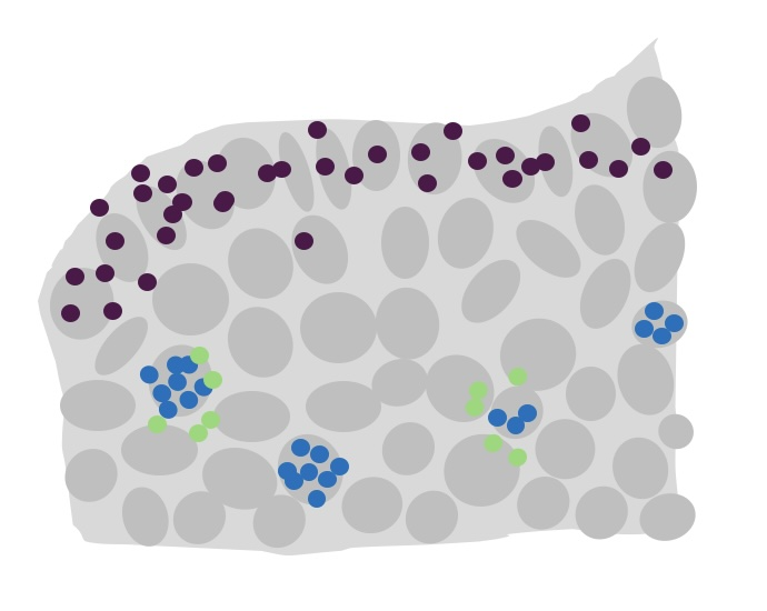
It is possible to test for genes that are expressed in a non-random spatial pattern. These might be restricted to regions of a tissue (e.g. epithelia), near structures or simply having very high expression in selected cells only (e.g. immunoglobulins in plasma cells).
One popular approach to find these genes is the MoransI test of spatial autocorrelation.
This example will show how to use the morans test within Seurat to find spatially restricted genes.
This requires:
- X,Y coordinates of individual transcripts, or their cells.
- Annotation of the tissue samples in the cell metadata (if multiple samples)
There is no need for celltype annotation.
For example:
- What cells are spatially restricted in this tissue due to some structure?
- Are some cancer-related genes showing a restricted spatial expression (and does this align with tumour-dense regions?)
Steps:
- Subset experiment to each tissue
- Calculate Moran’s I for each sample
- Join and inspect results
Worked example
Paper Microglia-astrocyte crosstalk in the amyloid plaque niche of an Alzheimer’s disease mouse model, as revealed by spatial transcriptomics(Mallach et al. 2024) explores the spatial transcription of amyloid plaques in a mouse model.
Their work includes an analysis of cosMx samples from of 4 mouse brain samples.
Those sections show very distinct spatial patterning of gene expression due to the different brain structures. This example will test which genes are expressed in a spatially restricted pattern, independently of any celltype annotations. e.g.
- Present within or nearby a given structure
- Existing in ‘clumps’ e.g. high expression on a small subset of cells
Load libraries and data
Load relevant libraries
# NB: The Rfast2 and ape packages may need to be installed
# to use the moransI test (in addition to Seurat)
# The GSL system library might also need to be installed, if it isn't already.
# install.packages('Rfast2')
# install.packages('ape')


library(Seurat)
library(tidyverse)
library(DT)


# Certain stps may result in error:
#Error in getGlobalsAndPackages(expr, envir = envir, globals = globals) :
#  The total size of the 14 globals exported for future expression (‘FUN()’) is 1.21 GiB.. This exceeds the maximum allowed size of 500.00 MiB (option 'future.globals.maxSize'). The three largest globals are ‘FUN’ (824.48 MiB of class ‘function’), ‘x’ (411.83 MiB of class ‘list’) and ‘over’ (940.20 KiB of class ‘function’)
# this can be fixed by increaseing the future.globals.maxsize variable (to an acceptable amount of ram)
options(future.globals.maxSize= 5*1024^3) # Set to 5Gb
And load the preprocessed Seurat object.
dataset_dir      <- '~/projects/spatialsnippets/datasets/GSE263793_Mallach2024_AlzPlaque/processed_data/'
seurat_file_01_preprocessed <- file.path(dataset_dir,  "GSE263793_AlzPlaque_seurat_01_preprocessed.RDS")

so <- readRDS(seurat_file_01_preprocessed)
Spatially variable features
Morans test can be slow to run, so save time by only running it on variable features. Variable features are those with a non-even distribution across cells, and are routinely deteced with FindVariableFeatures() during preprocessing. Non variable features are unlikely to be spatially restricted.
For the purpose of this demo, recalculate just the top 10 variable features. The actual number for a real experiment could be judged from the variable features plot below, e.g. 100-200-2000 (or whatever you use for PCA - it really depends on your panel!).
num_variable_features = 30 # Test only! Should be much larger. Consider using all your VariableFeatures used for UMAPs, et.c.
so <-  FindVariableFeatures(so, nfeatures=num_variable_features)
VariableFeaturePlot(so)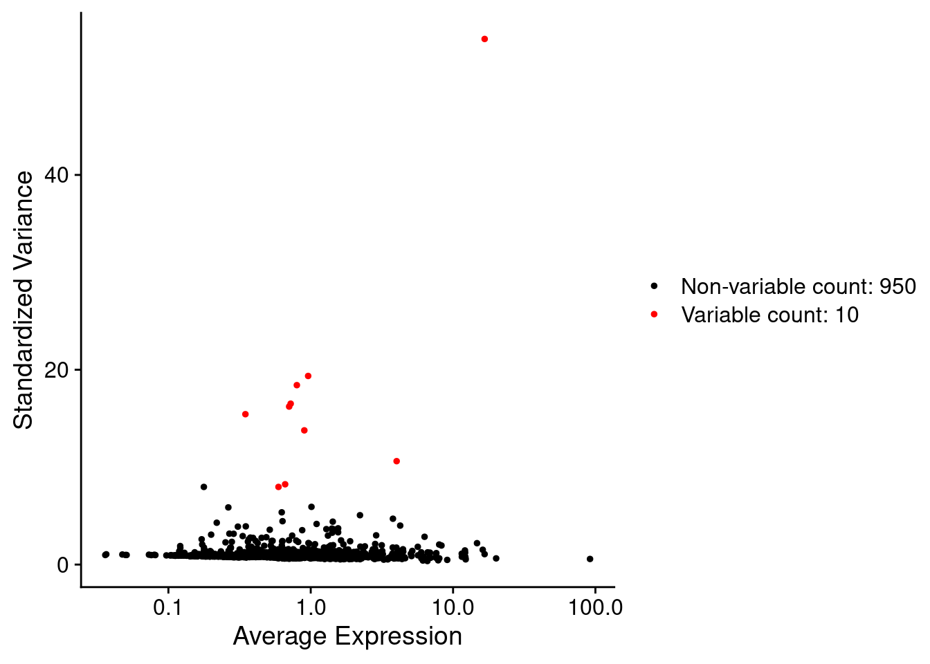
We will look for spatially variable features on each of our tissue samples independently; in this case 4 samples across 2 slides. But first, just test one.
We do this because all probes are essentially going to be restricted to the tissue itself, not the surrounding empty slide. This might be particularly noticeable on a panel of many small cores.
First, subset to just one tissue sample.
so.sample <- subset( so, subset= sample == 'sample1')Then find the spatially variable genes with FindSpatiallyVariableFeatures() function.
That code should look like this:
so.sample <- FindSpatiallyVariableFeatures(
  so.sample,
  assay = "RNA",
  features = VariableFeatures(so.sample),
  selection.method = "moransi",
  layer = "counts")
However, right now, there is a bug with the current FindSpatiallyVariableFeatures() function with this dataset. If you find the R code segfaults (ie. R exits entirely) with the message “address (nil), cause ‘memory not mapped’”, consider the workaroudn below. Also, check issue ticket here, it may be fixed.
so.sample.assay <- so.sample[['RNA']]
# Or equivalently
# so.sample.assay <- GetAssay(so.sample, "RNA")

# Make sure that the rownames of the coordinate table is the cell names
# Might not occur for certain types of data.
tc <- GetTissueCoordinates(so.sample)
rownames(tc)<- tc$cell

# When given an 'assay' FindSpatiallyVariableFeatures returns an assay. Put it back in the seurat object.
so.sample[['RNA']] <- FindSpatiallyVariableFeatures(
  so.sample.assay,
  layer = "scale.data",
  spatial.location = tc,
  features = VariableFeatures(so.sample),
  selection.method = "moransi",
  nfeatures=10 # mark top 10 spatially variable
  )
Resume
Now we have a a seurat object with the moransI scores embedded in the feature metatdata of the ‘RNA’ assay.
gene_metadata <- so.sample[["RNA"]]@meta.data
#NB: This is geme metadata, different to the usual *cell* metadata found at so.sample@meta.data
# so.sample[['RNA']]  retreives the 'RNA' assay.
DT::datatable(head(gene_metadata), width='100%')
The whole gene-metadata includes other columns, and in fact the columns we are interested in only have values for the ‘variable’ genes that we tested. So, make a summary table with just the relevant data.
gene_metadata_morans <-
  filter(gene_metadata, !is.na(moransi.spatially.variable.rank)) %>%
  select(feature,
         MoransI_observed, MoransI_p.value, moransi.spatially.variable,moransi.spatially.variable.rank) %>%
  arrange(moransi.spatially.variable.rank)

DT::datatable(gene_metadata_morans, width = '100%')
Plot results
We can pull out the most significant genes from that table.
top_genes = gene_metadata_morans$feature[1:3]
top_genes
[1] "Ptgds" "Apod" "Vtn" Here we are plotting the top 3 genes on that slide. Each has a different but clear reasons for being spatially restricted. Ptgds and Penk seem to be restricted to specific regions of the tissue. Wherease Drd4 seems to have high expression in a subset of cells - its proximity to itself also triggers the significance n the moransI test.
NB: Genes without any sort of spatial pattern (e.g negative controls) might still have some sort of moransI test significance - since they’re still restricted to the tissue itself, it isn’t random.
ImageDimPlot(so.sample,  fov = "AD2.AD3.CosMx",
             molecules = top_genes,
             group.by = 'sample', cols = c("grey30"), # Make all cells grey.
             boundaries = "segmentation",
             border.color = 'black', axes = T, crop=TRUE)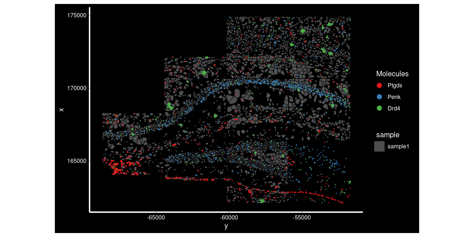
Run across all samples
Realistically, we would want to test all samples. Here we run the test on each tissue sample separately.
samples <- levels(so@meta.data$sample)
results_list <- list()

for (the_sample in samples) {

  so.sample <- subset( so, subset= sample == the_sample)

  # Again, this should be:
  #so.sample <- FindSpatiallyVariableFeatures(
  #  so.sample,
  #  assay = "RNA",
  #  features = VariableFeatures(so.sample),
  #  selection.method = "moransi",
  #  layer = "counts"
  #)

  # Workaround running FindSpatiallyVariableFeatures at the assay level
  so.sample.assay <- so.sample[['RNA']]
  tc <- GetTissueCoordinates(so.sample)
  rownames(tc)<- tc$cell

  # When given an 'assay' FindSpatiallyVariableFeatures returns an assay. Put it back in the seurat object.
  so.sample[['RNA']] <- FindSpatiallyVariableFeatures(
    so.sample.assay,
    layer = "scale.data",
    spatial.location = tc,
    features = VariableFeatures(so.sample),
    selection.method = "moransi",
    nfeatures=10 # mark top 10 spatially variable
    )
  # --- end workaround

  gene_metadata <- so.sample[["RNA"]]@meta.data
  results <-
  select(gene_metadata,
         feature,
         MoransI_observed,
         MoransI_p.value,
         moransi.spatially.variable,
         moransi.spatially.variable.rank) %>%
    filter(!is.na(moransi.spatially.variable.rank)) %>% # only tested
    arrange(moransi.spatially.variable.rank) %>%
    mutate(sample = the_sample) %>%
    select(sample, everything())


  results_list[[the_sample]] <- results
}

results_all <- bind_rows(results_list)
Display results for variable genes
DT::datatable(results_all, width='100%') Plot some of the moransI scores. We should keep in mind that the shape of the tissue itself limits where the targest can fall, but some genes are clearly more spatially restricted than others.
# unique set of genes that were top 10 morans in any sample
plot_genes <- filter(results_all, moransi.spatially.variable.rank <= 10) %>% pull(feature) %>% unique()
ggplot(filter(results_all, feature %in% plot_genes), aes(x=feature, y=MoransI_observed)) +
  geom_boxplot() +
  geom_point( mapping=aes(col=sample)) +
  theme_bw() +
  ggtitle("MoransI Per sample")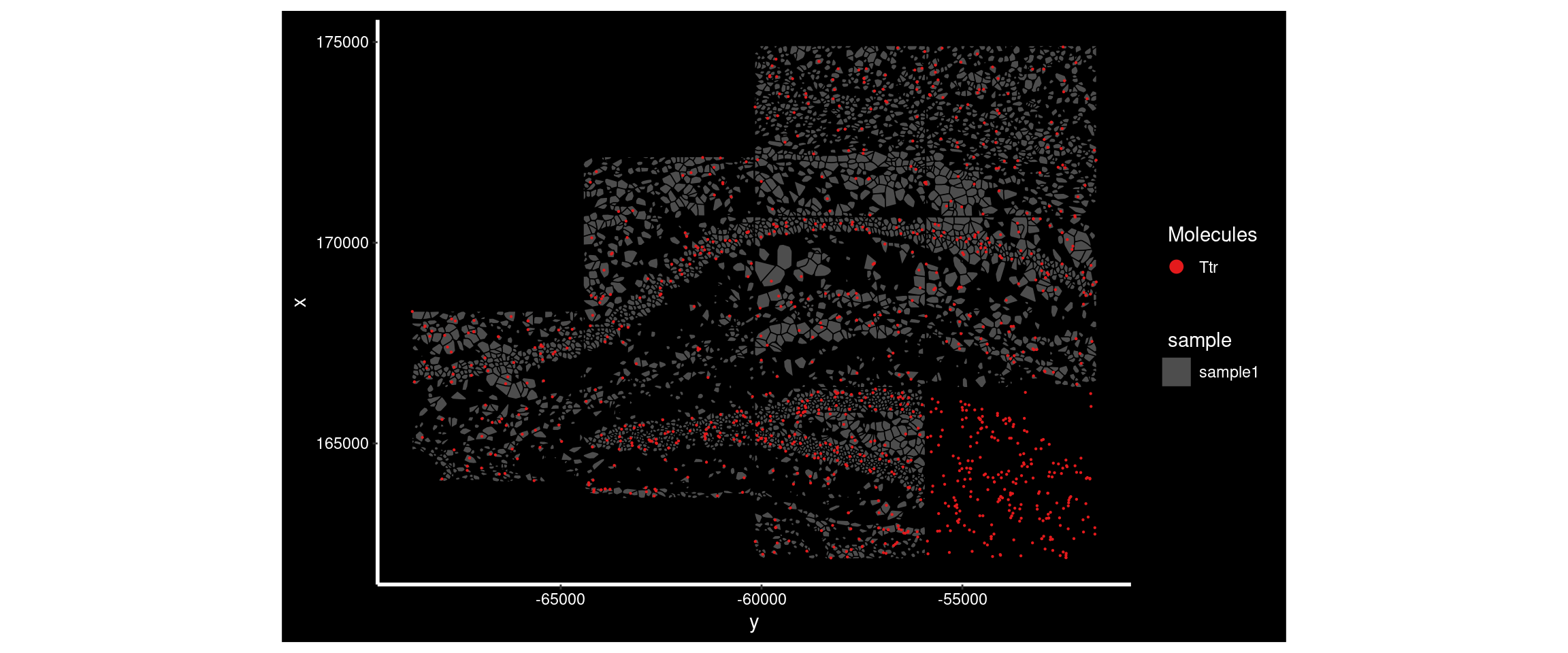
Check an example
Ttr had a much higher Moran’s I in sample4 than sample1. Plotting its distribution in both demonstrates the difference - there’s a very high expression region in sample4 not seen in sample1.
ImageDimPlot(
  subset( so, subset = sample == 'sample1'),
             fov          = "AD2.AD3.CosMx",
             molecules    = 'Ttr',
             group.by     = 'sample', cols = c("grey30"), # Make all cells grey.
             boundaries   = "segmentation",
             border.color = 'black', axes = T, crop=TRUE)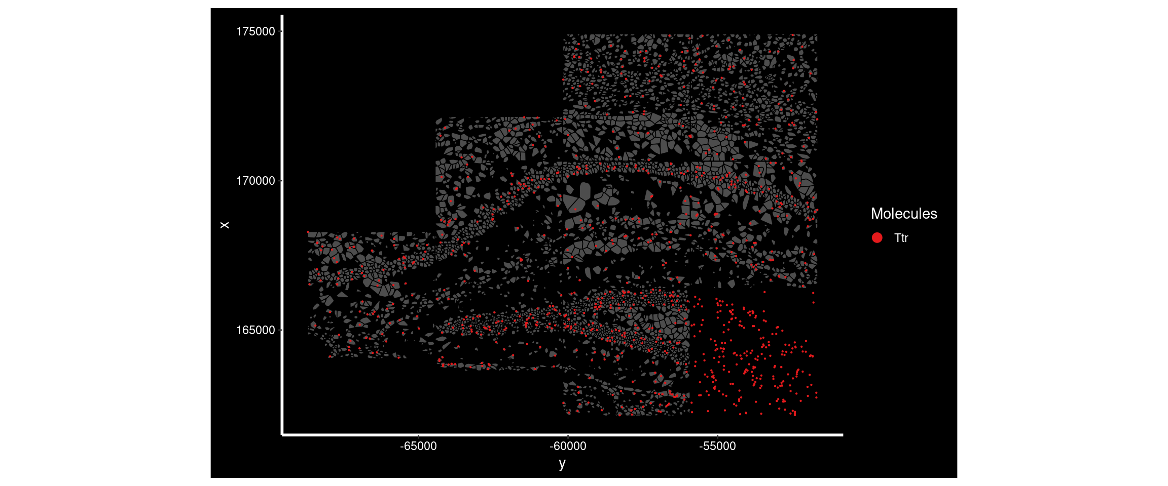
ImageDimPlot(
  subset( so, subset = sample == 'sample4'),
             fov          = "AD4.AD5.CosMx", # note the slide it is on.
             molecules    = 'Ttr',
             group.by     = 'sample', cols = c("grey30"), # Make all cells grey.
             boundaries   = "segmentation",
             border.color = 'black', axes = T, crop=TRUE)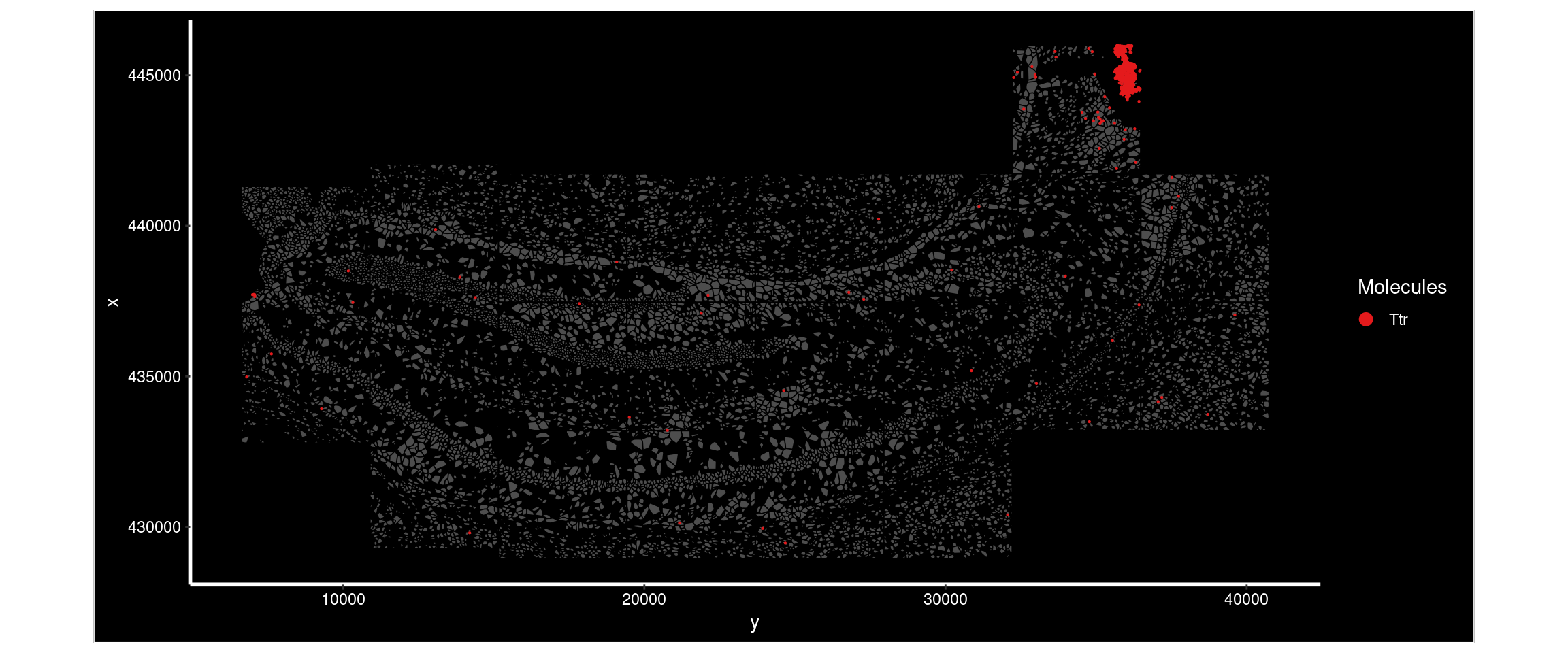
Code Snippet
Assumes that tissue samples are in a metadata column data called ‘sample’. If there are multiple slides, it may be neccessary to call joinlayers.
library(Seurat)
library(tidyverse)
library(DT)

## If not alread run, find variable features
#num_variable_features = 1000 # Choose based on likely results and acceptable runtime
#so <-  FindVariableFeatures(so, nfeatures=num_variable_features)


# Record moransI results for each sample, one by one.
samples <- unique(so@meta.data$sample)
results_list <- list()
for (the_sample in samples) {

  so.sample <- subset( so, subset= sample == the_sample)


  # TRY THIS FIRST
  # This is the Seurat method, and may have been fixed.
  #so.sample <- FindSpatiallyVariableFeatures(
  #  so.sample,
  #  assay = "RNA",
  #  features = VariableFeatures(so.sample),
  #  selection.method = "moransi",
  #  layer = "counts"
  #)

  # workaround
  # If the Seurat method above crashes (segfault), a workaround is
  # funning FindSpatiallyVariableFeatures at the assay level
  so.sample.assay <- so.sample[['RNA']]
  tc <- GetTissueCoordinates(so.sample)
  rownames(tc)<- tc$cell
  # When given an 'assay' FindSpatiallyVariableFeatures returns an assay. Put it back in the seurat object.
  so.sample[['RNA']] <- FindSpatiallyVariableFeatures(
    so.sample.assay,
    layer = "scale.data",
    spatial.location = tc,
    features = VariableFeatures(so.sample),
    selection.method = "moransi",
    nfeatures=10 # mark top 10 spatially variable
    )
  # --- end workaround


  # Format output table
  so.sample[["RNA"]]@meta.data$feature <- rownames(so.sample[["RNA"]])
  gene_metadata <- so.sample[["RNA"]]@meta.data
  results <-
  select(gene_metadata,
         feature,
         MoransI_observed,
         MoransI_p.value,
         moransi.spatially.variable,
         moransi.spatially.variable.rank) %>%
    filter(!is.na(moransi.spatially.variable.rank)) %>% # only tested
    arrange(moransi.spatially.variable.rank) %>%
    mutate(sample = the_sample) %>%
    select(sample, everything())


  results_list[[the_sample]] <- results
}

# Collect output result
results_all <- bind_rows(results_list)
Results
DT::datatable(results_all, width='100%')- sample: (not a default column, added by code): What tissue sample the test was run on.
- feature : The gene being tested
- MoransI_observed : The moransI statistic calculated. Higher values indicate more spatial correlation, 0 is completely random, and negative values indicate anti-correlation (ie repulsion).
- MoransI_p.value : P-value for the moransI test.
- moransi.spatially.variable : Is this gene spatially restricted? True or false value. The number of TRUEs is controlled by the nfeatures parameter of FindSpatiallyVariableFeatures.
- moransi.spatially.variable.rank : Ranking of the genes by spatial correlation, where 1 is the most distincly spatially restricted.
More information
- Microglia-astrocyte crosstalk in the amyloid plaque niche of an Alzheimer’s disease mouse model, as revealed by spatial transcriptomics: Data used in this example. (Mallach et al. 2024)
- MoransI wikipedia: What is MoransI test, with pictures.
- Seurat Spatially variable features: This is actually the sequencing based technology vignette (for visium data), but it covers the FindSpatiallyVariableFeatures function
- FindSpatiallyVariableFeatures() Bug report : Link to the bug report on the Seurat repo in github. Can check the status of this issue here.
- Voyager toolkit - spatial statistics for cosmx vignette : Here is a more focussed and detailed vignette on calculating spatial statistics for gene expression using the Voyager package. It does not use Seurat objects, it is rather using the bioconductor-compatible SpatialExperiment class.
References
sessionInfo()R version 4.4.0 (2024-04-24)
Platform: x86_64-pc-linux-gnu
Running under: Ubuntu 22.04.5 LTS
Matrix products: default
BLAS: /usr/lib/x86_64-linux-gnu/openblas-pthread/libblas.so.3
LAPACK: /usr/lib/x86_64-linux-gnu/openblas-pthread/libopenblasp-r0.3.20.so; LAPACK version 3.10.0
locale:
[1] LC_CTYPE=en_AU.UTF-8 LC_NUMERIC=C
[3] LC_TIME=en_AU.UTF-8 LC_COLLATE=en_AU.UTF-8
[5] LC_MONETARY=en_AU.UTF-8 LC_MESSAGES=en_AU.UTF-8
[7] LC_PAPER=en_AU.UTF-8 LC_NAME=C
[9] LC_ADDRESS=C LC_TELEPHONE=C
[11] LC_MEASUREMENT=en_AU.UTF-8 LC_IDENTIFICATION=C
time zone: Etc/UTC
tzcode source: system (glibc)
attached base packages:
[1] stats graphics grDevices datasets utils methods base
other attached packages:
[1] DT_0.33 lubridate_1.9.4 forcats_1.0.0 stringr_1.5.1
[5] dplyr_1.1.4 purrr_1.0.2 readr_2.1.5 tidyr_1.3.1
[9] tibble_3.2.1 ggplot2_3.5.1 tidyverse_2.0.0 Seurat_5.3.0
[13] SeuratObject_5.2.0 sp_2.2-0 workflowr_1.7.1
loaded via a namespace (and not attached):
[1] RColorBrewer_1.1-3 rstudioapi_0.17.1 jsonlite_1.8.9
[4] magrittr_2.0.3 spatstat.utils_3.1-2 farver_2.1.2
[7] rmarkdown_2.29 fs_1.6.5 vctrs_0.6.5
[10] ROCR_1.0-11 spatstat.explore_3.3-4 htmltools_0.5.8.1
[13] sass_0.4.9 sctransform_0.4.1 parallelly_1.42.0
[16] KernSmooth_2.23-26 bslib_0.9.0 htmlwidgets_1.6.4
[19] ica_1.0-3 plyr_1.8.9 plotly_4.10.4
[22] zoo_1.8-12 cachem_1.1.0 whisker_0.4.1
[25] igraph_2.1.4 mime_0.12 lifecycle_1.0.4
[28] pkgconfig_2.0.3 Matrix_1.7-4 R6_2.5.1
[31] fastmap_1.2.0 fitdistrplus_1.2-2 future_1.34.0
[34] shiny_1.10.0 digest_0.6.37 colorspace_2.1-1
[37] patchwork_1.3.0 ps_1.8.1 rprojroot_2.0.4
[40] tensor_1.5 RSpectra_0.16-2 irlba_2.3.5.1
[43] crosstalk_1.2.1 labeling_0.4.3 progressr_0.15.1
[46] timechange_0.3.0 spatstat.sparse_3.1-0 httr_1.4.7
[49] polyclip_1.10-7 abind_1.4-8 compiler_4.4.0
[52] proxy_0.4-27 withr_3.0.2 DBI_1.2.3
[55] fastDummies_1.7.5 MASS_7.3-64 classInt_0.4-11
[58] units_0.8-5 tools_4.4.0 lmtest_0.9-40
[61] httpuv_1.6.15 future.apply_1.11.3 Rfast2_0.1.5.4
[64] goftest_1.2-3 glue_1.8.0 callr_3.7.6
[67] nlme_3.1-166 promises_1.3.2 sf_1.0-19
[70] grid_4.4.0 Rtsne_0.17 getPass_0.2-4
[73] cluster_2.1.8 reshape2_1.4.4 generics_0.1.3
[76] gtable_0.3.6 spatstat.data_3.1-4 tzdb_0.4.0
[79] class_7.3-23 hms_1.1.3 data.table_1.16.4
[82] spatstat.geom_3.3-5 RcppAnnoy_0.0.22 ggrepel_0.9.6
[85] RANN_2.6.2 pillar_1.10.1 spam_2.11-1
[88] RcppHNSW_0.6.0 later_1.4.1 splines_4.4.0
[91] lattice_0.22-6 renv_1.0.5 survival_3.8-3
[94] deldir_2.0-4 tidyselect_1.2.1 Rnanoflann_0.0.3
[97] miniUI_0.1.1.1 pbapply_1.7-2 knitr_1.49
[100] git2r_0.33.0 gridExtra_2.3 scattermore_1.2
[103] xfun_0.50 matrixStats_1.5.0 stringi_1.8.4
[106] lazyeval_0.2.2 yaml_2.3.10 evaluate_1.0.3
[109] codetools_0.2-20 BiocManager_1.30.25 cli_3.6.3
[112] RcppParallel_5.1.11-1 uwot_0.2.2 xtable_1.8-4
[115] reticulate_1.40.0 munsell_0.5.1 processx_3.8.5
[118] jquerylib_0.1.4 Rcpp_1.0.14 zigg_0.0.2
[121] globals_0.16.3 spatstat.random_3.3-2 png_0.1-8
[124] Rfast_2.1.5.1 spatstat.univar_3.1-1 parallel_4.4.0
[127] dotCall64_1.2 listenv_0.9.1 viridisLite_0.4.2
[130] e1071_1.7-16 scales_1.3.0 ggridges_0.5.6
[133] rlang_1.1.5 cowplot_1.1.3