9 Cluster Markers
9.1 Finding differentially expressed features (cluster biomarkers)
Seurat can help you find markers that define clusters via differential expression. By default, it identifies positive and negative markers of a single cluster (specified in ident.1), compared to all other cells. FindAllMarkers() automates this process for all clusters, but you can also test groups of clusters vs. each other, or against all cells.
The min.pct argument requires a feature to be detected at a minimum percentage in either of the two groups of cells, and the thresh.test argument requires a feature to be differentially expressed (on average) by some amount between the two groups. You can set both of these to 0, but with a dramatic increase in time - since this will test a large number of features that are unlikely to be highly discriminatory. As another option to speed up these computations, max.cells.per.ident can be set. This will downsample each identity class to have no more cells than whatever this is set to. While there is generally going to be a loss in power, the speed increases can be significant and the most highly differentially expressed features will likely still rise to the top.
# find all markers of cluster 2
cluster2.markers <- FindMarkers(pbmc, ident.1 = 2, min.pct = 0.25)
head(cluster2.markers, n = 5)
#>             p_val avg_log2FC pct.1 pct.2    p_val_adj
#> IL32 2.892340e-90  1.2013522 0.947 0.465 3.966555e-86
#> LTB  1.060121e-86  1.2695776 0.981 0.643 1.453850e-82
#> CD3D 8.794641e-71  0.9389621 0.922 0.432 1.206097e-66
#> IL7R 3.516098e-68  1.1873213 0.750 0.326 4.821977e-64
#> LDHB 1.642480e-67  0.8969774 0.954 0.614 2.252497e-63
# find all markers distinguishing cluster 5 from clusters 0 and 3
cluster5.markers <- FindMarkers(pbmc, ident.1 = 5, ident.2 = c(0, 3), min.pct = 0.25)
head(cluster5.markers, n = 5)
#>                       p_val avg_log2FC pct.1 pct.2
#> FCGR3A        8.246578e-205   4.261495 0.975 0.040
#> IFITM3        1.677613e-195   3.879339 0.975 0.049
#> CFD           2.401156e-193   3.405492 0.938 0.038
#> CD68          2.900384e-191   3.020484 0.926 0.035
#> RP11-290F20.3 2.513244e-186   2.720057 0.840 0.017
#>                   p_val_adj
#> FCGR3A        1.130936e-200
#> IFITM3        2.300678e-191
#> CFD           3.292945e-189
#> CD68          3.977587e-187
#> RP11-290F20.3 3.446663e-182
# find markers for every cluster compared to all remaining cells, report only the positive ones
pbmc.markers <- FindAllMarkers(pbmc, only.pos = TRUE, min.pct = 0.25, logfc.threshold = 0.25)
#> Calculating cluster 0
#> Calculating cluster 1
#> Calculating cluster 2
#> Calculating cluster 3
#> Calculating cluster 4
#> Calculating cluster 5
#> Calculating cluster 6
#> Calculating cluster 7
#> Calculating cluster 8
pbmc.markers %>% group_by(cluster) %>% slice_max(n = 2, order_by = avg_log2FC)
#> # A tibble: 18 × 7
#> # Groups:   cluster [9]
#>        p_val avg_log2FC pct.1 pct.2 p_val_adj cluster gene
#>        <dbl>      <dbl> <dbl> <dbl>     <dbl> <fct>   <chr>
#>  1 9.57e- 88       1.36 0.447 0.108 1.31e- 83 0       CCR7
#>  2 3.75e-112       1.09 0.912 0.592 5.14e-108 0       LDHB
#>  3 0               5.57 0.996 0.215 0         1       S100A9
#>  4 0               5.48 0.975 0.121 0         1       S100A8
#>  5 1.06e- 86       1.27 0.981 0.643 1.45e- 82 2       LTB
#>  6 2.97e- 58       1.23 0.42  0.111 4.07e- 54 2       AQP3
#>  7 0               4.31 0.936 0.041 0         3       CD79A
#>  8 9.48e-271       3.59 0.622 0.022 1.30e-266 3       TCL1A
#>  9 5.61e-202       3.10 0.983 0.234 7.70e-198 4       CCL5
#> 10 7.25e-165       3.00 0.577 0.055 9.95e-161 4       GZMK
#> 11 3.51e-184       3.31 0.975 0.134 4.82e-180 5       FCGR3A
#> 12 2.03e-125       3.09 1     0.315 2.78e-121 5       LST1
#> 13 3.13e-191       5.32 0.961 0.131 4.30e-187 6       GNLY
#> 14 7.95e-269       4.83 0.961 0.068 1.09e-264 6       GZMB
#> 15 1.48e-220       3.87 0.812 0.011 2.03e-216 7       FCER1A
#> 16 1.67e- 21       2.87 1     0.513 2.28e- 17 7       HLA-D…
#> 17 1.92e-102       8.59 1     0.024 2.63e- 98 8       PPBP
#> 18 9.25e-186       7.29 1     0.011 1.27e-181 8       PF4
Seurat has several tests for differential expression which can be set with the test.use parameter (see our DE vignette for details). For example, the ROC test returns the ‘classification power’ abs(AUC-0.5)*2 for any individual marker, ranging from 0 = random to 1 = perfect.
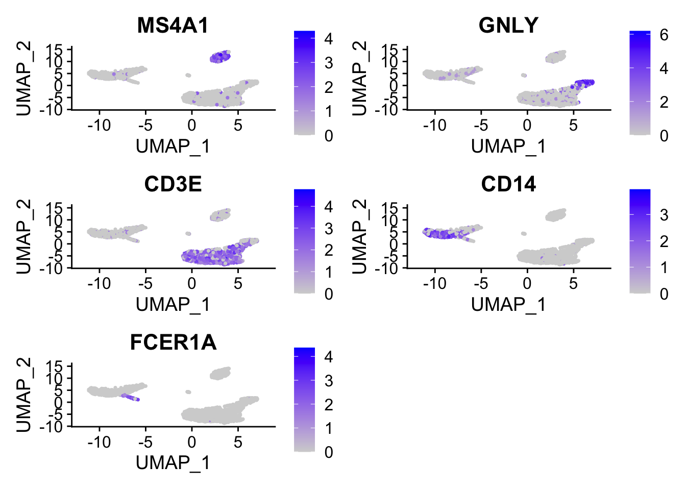
cluster0.markers <- FindMarkers(pbmc, ident.1 = 0, logfc.threshold = 0.25, test.use = "roc", only.pos = TRUE)We include several tools for visualizing marker expression. VlnPlot() (shows expression probability distributions across clusters), and FeaturePlot() (visualizes feature expression on a tSNE or PCA plot) are our most commonly used visualizations. We also suggest exploring RidgePlot(), CellScatter(), and DotPlot() as additional methods to view your dataset.
# you can plot raw counts as well
VlnPlot(pbmc, features = c("NKG7", "PF4"), slot = 'counts', log = TRUE)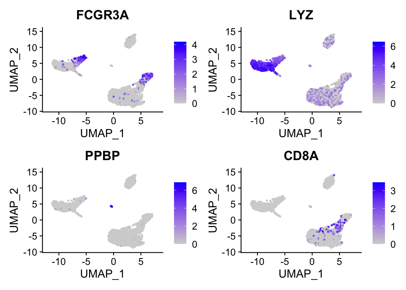
FeaturePlot(pbmc, features = c("MS4A1", "GNLY", "CD3E", "CD14", "FCER1A", "FCGR3A", "LYZ", "PPBP", "CD8A"))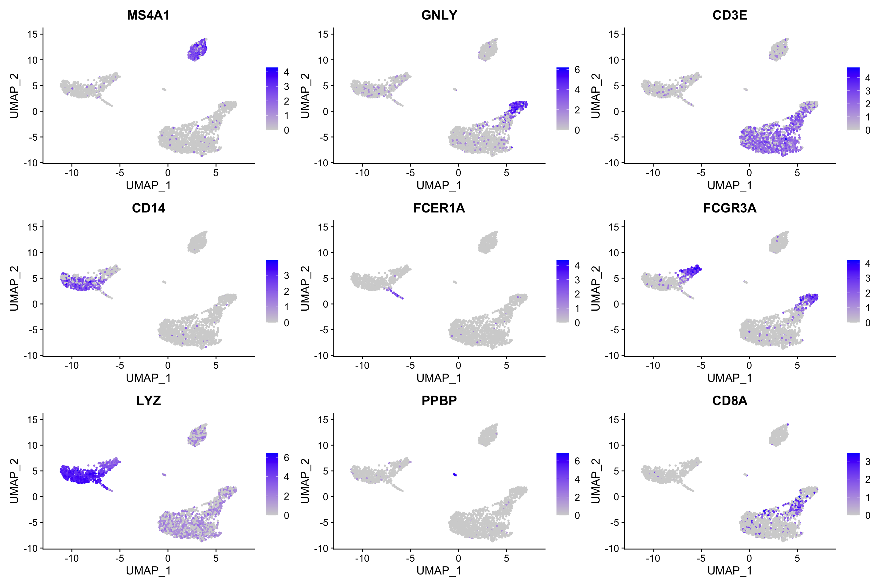
Other useful plots
These are ridgeplots, cell scatter plots and dotplots. Replace FeaturePlot with the other functions.
RidgePlot(pbmc, features = c("MS4A1", "GNLY", "CD3E", "CD14", "FCER1A", "FCGR3A", "LYZ", "PPBP", "CD8A"))
#> Picking joint bandwidth of 0.0236
#> Picking joint bandwidth of 0.0859
#> Picking joint bandwidth of 0.126
#> Picking joint bandwidth of 0.0337
#> Picking joint bandwidth of 0.0659
#> Picking joint bandwidth of 0.0582
#> Picking joint bandwidth of 0.309
#> Picking joint bandwidth of 0.0156
#> Picking joint bandwidth of 0.0366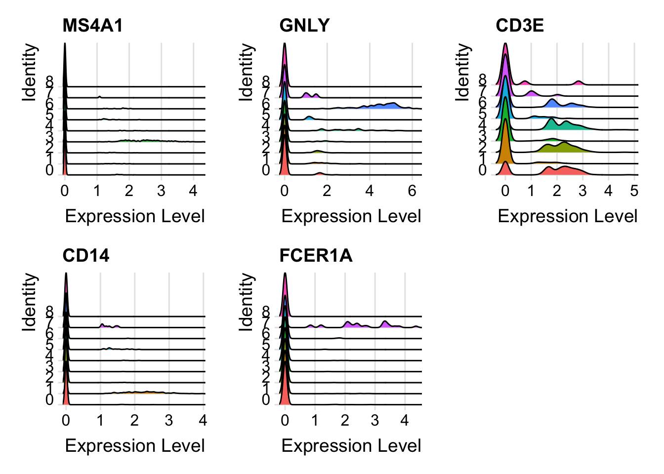 For CellScatter plots, will need the cell id of the cells you want to look at. You can get this from the cell metadata (
pbmc@meta.data).
head( pbmc@meta.data )
#>                  orig.ident nCount_RNA nFeature_RNA
#> AAACATACAACCAC-1     pbmc3k       2419          779
#> AAACATTGAGCTAC-1     pbmc3k       4903         1352
#> AAACATTGATCAGC-1     pbmc3k       3147         1129
#> AAACCGTGCTTCCG-1     pbmc3k       2639          960
#> AAACCGTGTATGCG-1     pbmc3k        980          521
#> AAACGCACTGGTAC-1     pbmc3k       2163          781
#>                  percent.mt RNA_snn_res.0.5 seurat_clusters
#> AAACATACAACCAC-1  3.0177759               2               6
#> AAACATTGAGCTAC-1  3.7935958               3               1
#> AAACATTGATCAGC-1  0.8897363               2               0
#> AAACCGTGCTTCCG-1  1.7430845               1               5
#> AAACCGTGTATGCG-1  1.2244898               6               8
#> AAACGCACTGGTAC-1  1.6643551               2               0
#>                  RNA_snn_res.0.1 RNA_snn_res.0.2
#> AAACATACAACCAC-1               0               0
#> AAACATTGAGCTAC-1               3               3
#> AAACATTGATCAGC-1               0               0
#> AAACCGTGCTTCCG-1               1               1
#> AAACCGTGTATGCG-1               2               2
#> AAACGCACTGGTAC-1               0               0
#>                  RNA_snn_res.0.3 RNA_snn_res.0.4
#> AAACATACAACCAC-1               0               2
#> AAACATTGAGCTAC-1               3               3
#> AAACATTGATCAGC-1               0               2
#> AAACCGTGCTTCCG-1               1               1
#> AAACCGTGTATGCG-1               2               6
#> AAACGCACTGGTAC-1               0               2
#>                  RNA_snn_res.0.6 RNA_snn_res.0.7
#> AAACATACAACCAC-1               1               1
#> AAACATTGAGCTAC-1               3               3
#> AAACATTGATCAGC-1               1               1
#> AAACCGTGCTTCCG-1               2               2
#> AAACCGTGTATGCG-1               6               6
#> AAACGCACTGGTAC-1               1               1
#>                  RNA_snn_res.0.8 RNA_snn_res.0.9
#> AAACATACAACCAC-1               6               1
#> AAACATTGAGCTAC-1               2               2
#> AAACATTGATCAGC-1               1               1
#> AAACCGTGCTTCCG-1               4               4
#> AAACCGTGTATGCG-1               8               7
#> AAACGCACTGGTAC-1               1               1
#>                  RNA_snn_res.1 RNA_snn_res.1.1
#> AAACATACAACCAC-1             6               6
#> AAACATTGAGCTAC-1             2               2
#> AAACATTGATCAGC-1             1               1
#> AAACCGTGCTTCCG-1             4               4
#> AAACCGTGTATGCG-1             8               8
#> AAACGCACTGGTAC-1             1               1
#>                  RNA_snn_res.1.2 RNA_snn_res.1.3
#> AAACATACAACCAC-1               6               8
#> AAACATTGAGCTAC-1               2               2
#> AAACATTGATCAGC-1               1               0
#> AAACCGTGCTTCCG-1               4               5
#> AAACCGTGTATGCG-1               8               9
#> AAACGCACTGGTAC-1               1               0
#>                  RNA_snn_res.1.4 RNA_snn_res.1.5
#> AAACATACAACCAC-1               8               9
#> AAACATTGAGCTAC-1               2               2
#> AAACATTGATCAGC-1               0               1
#> AAACCGTGCTTCCG-1               5               4
#> AAACCGTGTATGCG-1               9               8
#> AAACGCACTGGTAC-1               0               1
#>                  RNA_snn_res.1.6 RNA_snn_res.1.7
#> AAACATACAACCAC-1               8               8
#> AAACATTGAGCTAC-1               1               1
#> AAACATTGATCAGC-1               0               0
#> AAACCGTGCTTCCG-1               3               3
#> AAACCGTGTATGCG-1               7               7
#> AAACGCACTGGTAC-1               0               0
#>                  RNA_snn_res.1.8 RNA_snn_res.1.9
#> AAACATACAACCAC-1               7               6
#> AAACATTGAGCTAC-1               1               1
#> AAACATTGATCAGC-1               0               0
#> AAACCGTGCTTCCG-1               3               3
#> AAACCGTGTATGCG-1               8               8
#> AAACGCACTGGTAC-1               0               0
#>                  RNA_snn_res.2
#> AAACATACAACCAC-1             6
#> AAACATTGAGCTAC-1             1
#> AAACATTGATCAGC-1             0
#> AAACCGTGCTTCCG-1             5
#> AAACCGTGTATGCG-1             8
#> AAACGCACTGGTAC-1             0
CellScatter(pbmc, cell1 = "AAACATACAACCAC-1", cell2 = "AAACATTGAGCTAC-1")
DotPlots
DotPlot(pbmc, features = c("MS4A1", "GNLY", "CD3E", "CD14", "FCER1A", "FCGR3A", "LYZ", "PPBP", "CD8A"))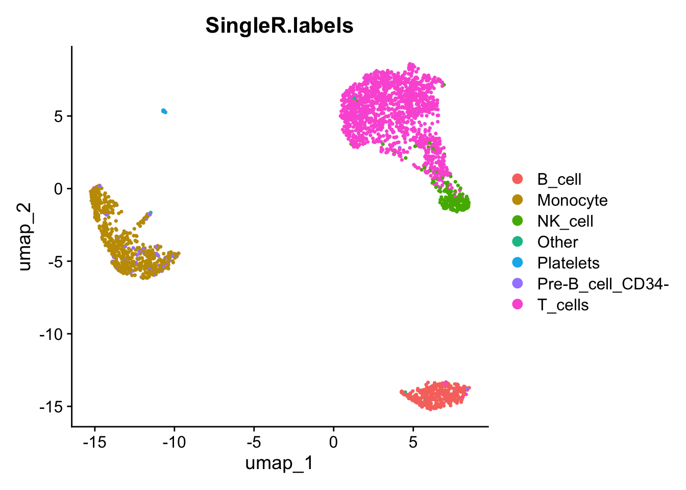
Which plots do you prefer? Discuss.
DoHeatmap() generates an expression heatmap for given cells and features. In this case, we are plotting the top 20 markers (or all markers if less than 20) for each cluster.
top10 <- pbmc.markers %>% group_by(cluster) %>% top_n(n = 10, wt = avg_log2FC)
DoHeatmap(pbmc, features = top10$gene) + NoLegend()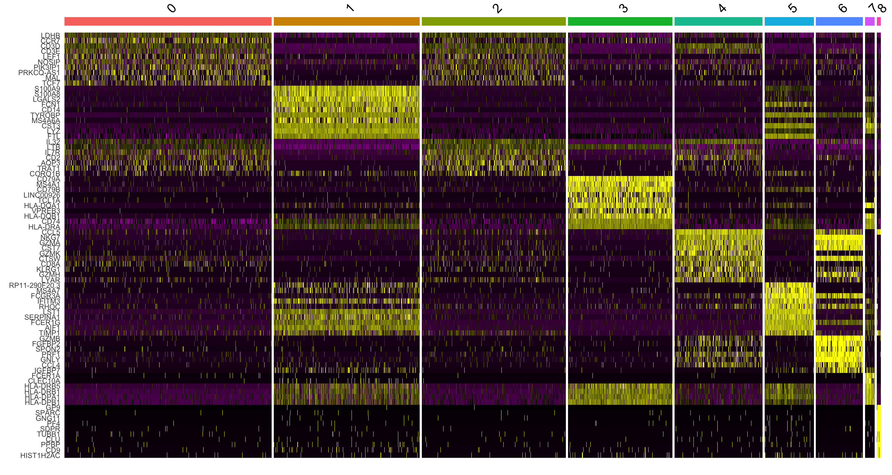
9.2 Assigning cell type identity to clusters
Fortunately in the case of this dataset, we can use canonical markers to easily match the unbiased clustering to known cell types:
| Cluster ID | Markers | Cell Type |
|---|---|---|
| 0 | IL7R, CCR7 | Naive CD4+ T |
| 1 | CD14, LYZ | CD14+ Mono |
| 2 | IL7R, S100A4 | Memory CD4+ |
| 3 | MS4A1 | B |
| 4 | CD8A | CD8+ T |
| 5 | FCGR3A, MS4A7 | FCGR3A+ Mono |
| 6 | GNLY, NKG7 | NK |
| 7 | FCER1A, CST3 | DC |
| 8 | PPBP | Platelet |
new.cluster.ids <- c("Naive CD4 T", "CD14+ Mono", "Memory CD4 T", "B", "CD8 T", "FCGR3A+ Mono", "NK", "DC", "Platelet")
names(new.cluster.ids) <- levels(pbmc)
pbmc <- RenameIdents(pbmc, new.cluster.ids)
DimPlot(pbmc, reduction = 'umap', label = TRUE, pt.size = 0.5) + NoLegend()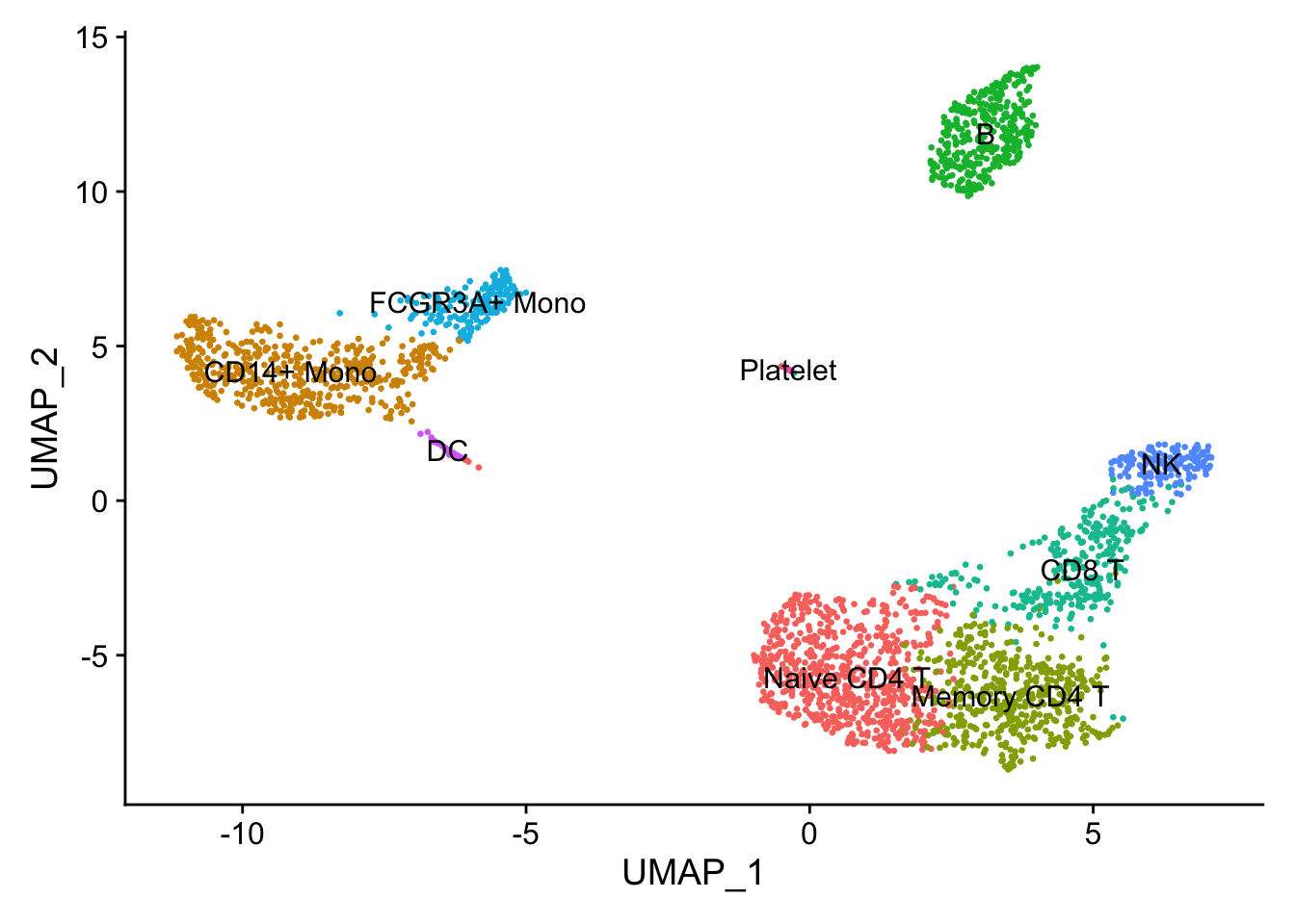
saveRDS(pbmc, file = "pbmc3k_final.rds")