7 Differential Expression
There are many different methods for calculating differential expression between groups in scRNAseq data. There are a number of review papers worth consulting on this topic.
There is the Seurat differential expression Vignette which walks through the variety implemented in Seurat.
There is also a good discussion of useing pseudobulk approaches which is worth checking out if youre planning differential expression analyses.
We will now look at GSE96583, another PBMC dataset. For speed, we will be looking at a subset of 5000 cells from this data. The cells in this dataset were pooled from eight individual donors. This data contains two batches of single cell sequencing. One of the batches was stimulated with IFN-beta.
The data has already been processed as we have done with the first PBMC dataset, and can be loaded from the kang2018.rds file in the data folder.
kang <- readRDS("data/kang2018.rds")
head(kang@meta.data)
#>                     orig.ident nCount_RNA nFeature_RNA  ind
#> AGGGCGCTATTTCC-1 SeuratProject       2020          523 1256
#> GGAGACGATTCGTT-1 SeuratProject        840          381 1256
#> CACCGTTGTCGTAG-1 SeuratProject       3097          995 1016
#> TATCGTACACGCAT-1 SeuratProject       1011          540 1488
#> TGACGCCTTGCTTT-1 SeuratProject        570          367  101
#> TACGAGACCTATTC-1 SeuratProject       2399          770 1244
#>                  stim              cell multiplets
#> AGGGCGCTATTTCC-1 stim   CD14+ Monocytes    singlet
#> GGAGACGATTCGTT-1 stim       CD4 T cells    singlet
#> CACCGTTGTCGTAG-1 ctrl FCGR3A+ Monocytes    singlet
#> TATCGTACACGCAT-1 stim           B cells    singlet
#> TGACGCCTTGCTTT-1 ctrl       CD4 T cells       ambs
#> TACGAGACCTATTC-1 stim       CD4 T cells    singlet
How cells from each condition do we have?
table(kang$stim)
#>
#> ctrl stim
#> 2449 2551
How many cells per individuals per group?
table(kang$ind, kang$stim)
#>
#>        ctrl stim
#>   101   178  229
#>   107   117  107
#>   1015  514  496
#>   1016  356  356
#>   1039  100  118
#>   1244  380  313
#>   1256  394  390
#>   1488  410  542
And for each sample, how many of each cell type has been classified?
table(paste(kang$ind,kang$stim), kang$cell)
#>
#>             B cells CD14+ Monocytes CD4 T cells CD8 T cells
#>   101 ctrl       24              48          61          15
#>   101 stim       30              52          84          17
#>   1015 ctrl      81             149         145          46
#>   1015 stim      68             151         150          22
#>   1016 ctrl      22              72          89         112
#>   1016 stim      29              65          66         115
#>   1039 ctrl       7              35          40           6
#>   1039 stim       7              28          51           6
#>   107 ctrl        9              51          32           6
#>   107 stim        9              35          43           1
#>   1244 ctrl      23              86         206           8
#>   1244 stim      18              58         191           4
#>   1256 ctrl      32              81         180          29
#>   1256 stim      42              70         198          25
#>   1488 ctrl      36              59         247          13
#>   1488 stim      59              59         325          15
#>
#>             Dendritic cells FCGR3A+ Monocytes
#>   101 ctrl                4                11
#>   101 stim                6                23
#>   1015 ctrl               4                50
#>   1015 stim              17                44
#>   1016 ctrl               4                22
#>   1016 stim               2                32
#>   1039 ctrl               1                 3
#>   1039 stim               1                 8
#>   107 ctrl                3                12
#>   107 stim                2                 5
#>   1244 ctrl               8                19
#>   1244 stim               6                 4
#>   1256 ctrl               6                20
#>   1256 stim               3                11
#>   1488 ctrl               8                25
#>   1488 stim              12                28
#>
#>             Megakaryocytes NK cells
#>   101 ctrl               4       11
#>   101 stim               1       16
#>   1015 ctrl              5       34
#>   1015 stim              5       39
#>   1016 ctrl              4       31
#>   1016 stim              1       46
#>   1039 ctrl              6        1
#>   1039 stim             10        5
#>   107 ctrl               1        3
#>   107 stim               0       12
#>   1244 ctrl              5       25
#>   1244 stim              4       28
#>   1256 ctrl              1       45
#>   1256 stim              8       33
#>   1488 ctrl              4       18
#>   1488 stim              6       38
7.1 Prefiltering
Why do we need to do this?
If expression is below a certain level, it will be almost impossible to see any differential expression.
When doing differential expression, you generally ignore genes with low expression. In single cell datasets, there are many genes like this. Filtering here to make our dataset smaller so it runs quicker, and there is less aggressive correction for multiple hypotheses.
How many genes before filtering?
kang
#> An object of class Seurat
#> 35635 features across 5000 samples within 1 assay
#> Active assay: RNA (35635 features, 2000 variable features)
#>  3 layers present: counts, data, scale.data
#>  2 dimensional reductions calculated: pca, umap
How many copies of each gene are there?
total_per_gene <- rowSums(GetAssayData(kang, 'RNA', layer = "counts")) #Make sure its RNA assay, layer = counts
hist(log10(total_per_gene))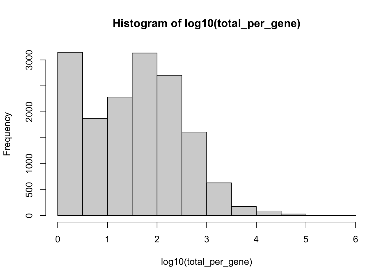
Lets keep only those genes with at least 50 copies across the entire experiment.
kang <- kang[total_per_gene >= 50, ] How many genes after filtering?
kang
#> An object of class Seurat
#> 7216 features across 5000 samples within 1 assay
#> Active assay: RNA (7216 features, 1228 variable features)
#>  3 layers present: counts, data, scale.data
#>  2 dimensional reductions calculated: pca, umap
We might like to see the effect of IFN-beta stimulation on each cell type individually. For the purposes of this workshop, just going to test one cell type; CD14+ Monocytes
An easy way is to subset the object.
kang.celltype <- kang[, kang$cell == "CD14+ Monocytes" ]
DimPlot(kang.celltype)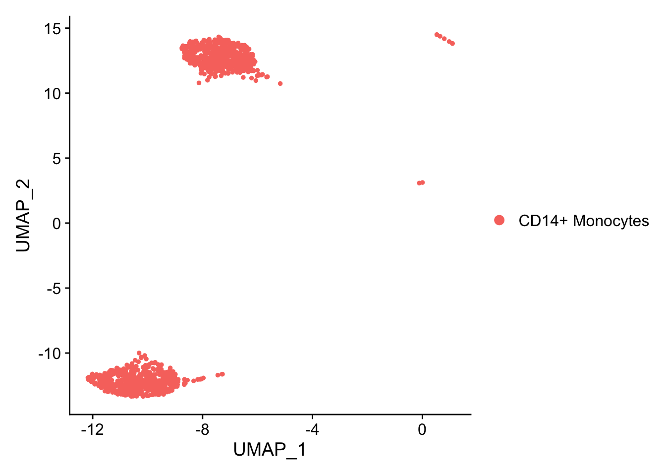
7.2 Default Wilcox test
To run this test, we change the Idents to the factor(column) we want to test. In this case, that’s ‘stim’.
# Change Ident to Condition
Idents(kang.celltype) <- kang.celltype$stim

# default, wilcox test
de_result_wilcox <- FindMarkers(kang.celltype,
            ident.1 = 'stim',
            ident.2 = 'ctrl',
            logfc.threshold = 0, # Give me ALL results
            min.pct = 0
            )
#> For a (much!) faster implementation of the Wilcoxon Rank Sum Test,
#> (default method for FindMarkers) please install the presto package
#> --------------------------------------------
#> install.packages('devtools')
#> devtools::install_github('immunogenomics/presto')
#> --------------------------------------------
#> After installation of presto, Seurat will automatically use the more
#> efficient implementation (no further action necessary).
#> This message will be shown once per session

# Add average expression for plotting

de_result_wilcox$AveExpr<- rowMeans(GetAssayData(kang.celltype,assay="RNA", layer = "data")[rownames(de_result_wilcox),])
Look at the top differentially expressed genes.
head(de_result_wilcox)
#>                 p_val avg_log2FC pct.1 pct.2     p_val_adj
#> RSAD2   5.541857e-197   6.807428 0.975 0.043 3.999004e-193
#> CXCL10  9.648067e-197   8.043584 0.973 0.038 6.962045e-193
#> IFIT3   4.988121e-196   6.232966 0.979 0.050 3.599428e-192
#> TNFSF10 1.116418e-195   6.567507 0.977 0.055 8.056075e-192
#> IFIT1   8.116699e-190   6.764859 0.950 0.026 5.857010e-186
#> ISG15   1.524836e-187   6.373685 0.998 0.320 1.100322e-183
#>          AveExpr
#> RSAD2   1.686530
#> CXCL10  2.388462
#> IFIT3   1.701247
#> TNFSF10 1.682688
#> IFIT1   1.584751
#> ISG15   3.239774
p1 <- ggplot(de_result_wilcox, aes(x=AveExpr, y=avg_log2FC, col=p_val_adj < 0.05)) +
  geom_point() +
  scale_colour_manual(values=c('TRUE'="red",'FALSE'="black")) +
  theme_bw() +
  ggtitle("Wilcox Test")


p2 <- ggplot(de_result_wilcox, aes(x=avg_log2FC, y=-log10(p_val), col=p_val_adj < 0.05)) +
  geom_point() +
  scale_colour_manual(values=c('TRUE'="red",'FALSE'="black")) +
  theme_bw() +
  ggtitle("Wilcox Test (Volcano)")

p1 + p2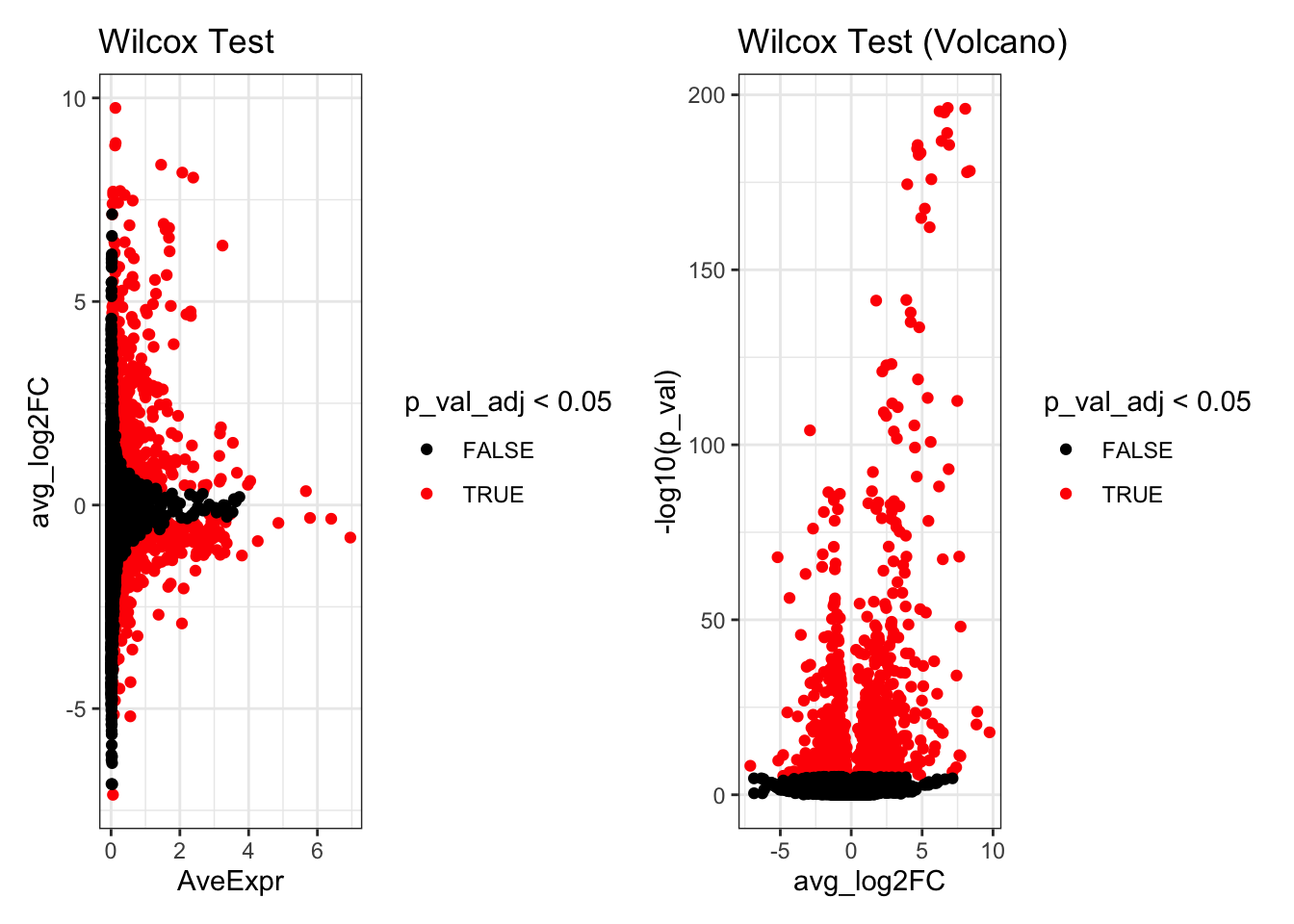
7.3 Seurat Negative binomial
Negative binonial test is run almost the same way - just need to specify it under ‘test.use’
# Change Ident to Condition
Idents(kang.celltype) <- kang.celltype$stim

# default, wilcox test
de_result_negbinom <- FindMarkers(kang.celltype,
            test.use="negbinom", # Choose a different test.
            ident.1 = 'stim',
            ident.2 = 'ctrl',
            logfc.threshold = 0, # Give me ALL results
            min.pct = 0
)

# Add average expression for plotting
de_result_negbinom$AveExpr<- rowMeans(GetAssayData(kang.celltype,assay="RNA", layer = "data")[rownames(de_result_negbinom),])
Look at the top differentially expressed genes.
head(de_result_negbinom)
#>          p_val avg_log2FC pct.1 pct.2 p_val_adj  AveExpr
#> CXCL10       0   8.043584 0.973 0.038         0 2.388462
#> CCL8         0   8.166731 0.909 0.022         0 2.071022
#> LY6E         0   4.891032 0.973 0.133         0 1.736931
#> APOBEC3A     0   4.755297 0.992 0.258         0 2.311961
#> IFITM3       0   4.683573 0.994 0.267         0 2.190185
#> IFI6         0   3.950817 0.979 0.253         0 1.820140
p1 <- ggplot(de_result_negbinom, aes(x=AveExpr, y=avg_log2FC, col=p_val_adj < 0.05)) +
  geom_point() +
  scale_colour_manual(values=c('TRUE'="red",'FALSE'="black")) +
  theme_bw() +
  ggtitle("Negative Bionomial Test")


p2 <- ggplot(de_result_negbinom, aes(x=avg_log2FC, y=-log10(p_val), col=p_val_adj < 0.05)) +
  geom_point() +
  scale_colour_manual(values=c('TRUE'="red",'FALSE'="black")) +
  theme_bw() +
  ggtitle("Negative Bionomial Test (Volcano)")

p1 + p2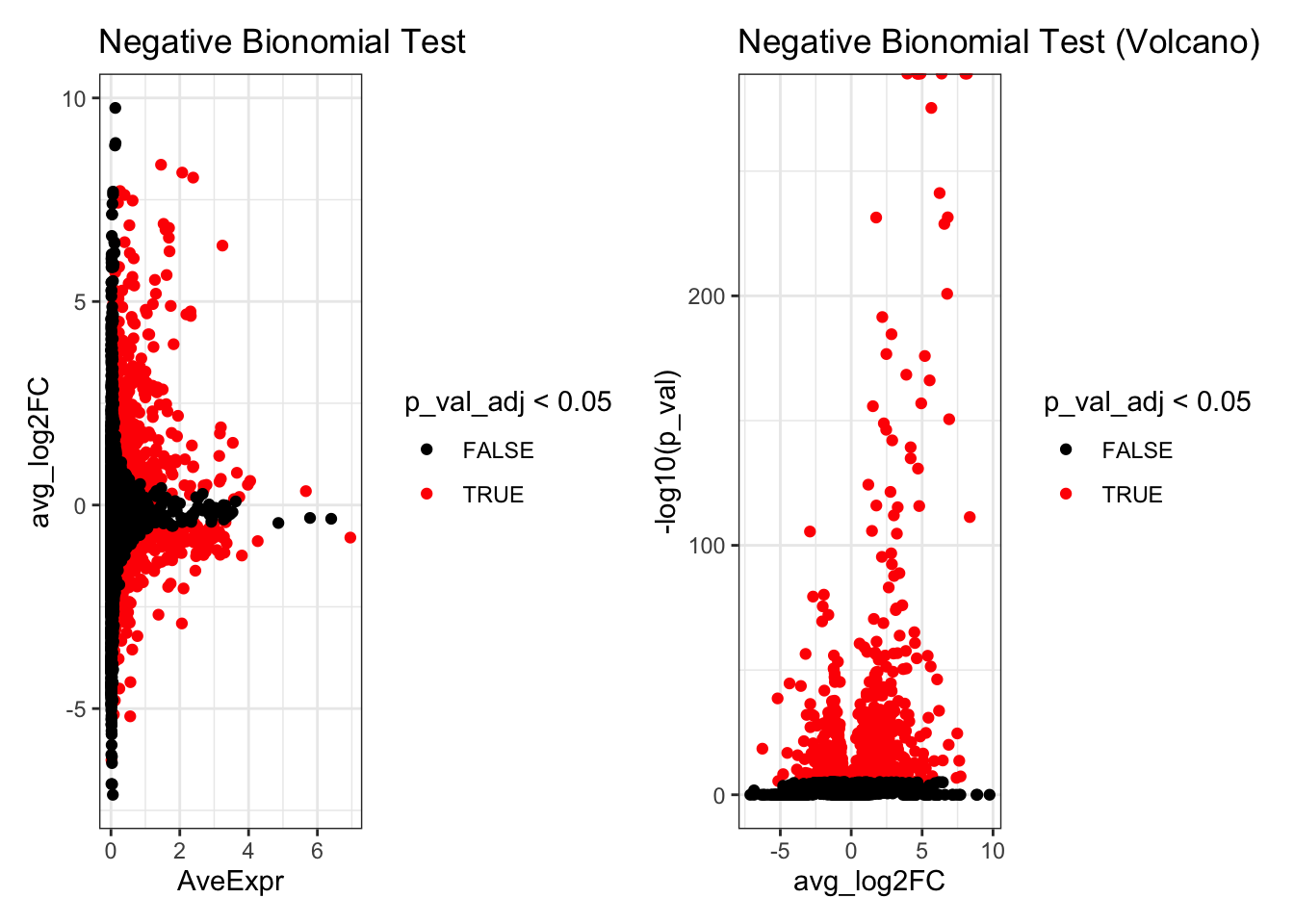
7.4 Pseudobulk
Pseudobulk analysis is an option where you have biological replicates. It is essentially pooling the individual cell counts and treating your expreiment like a bulk RNAseq.
First, you need to build a pseudobulk matrix - the AggregateExpression() function can do this, once you set the ‘Idents’ of your seurat object to your grouping factor (here, thats a combination of individual+treatment called ‘sample’, instead of the ‘stim’ treatment column).
# Tools for bulk differential expression
library(limma)
#>
#> Attaching package: 'limma'
#> The following object is masked from 'package:BiocGenerics':
#>
#>     plotMA
library(edgeR)
#>
#> Attaching package: 'edgeR'
#> The following object is masked from 'package:SingleCellExperiment':
#>
#>     cpm


# Change idents to ind for grouping.
kang.celltype$sample <- factor(paste(kang.celltype$stim, kang.celltype$ind, sep="_"))
Idents(kang.celltype) <- kang.celltype$sample

# THen pool together counts in those groups
# AggregateExperssion returns a list of matricies - one for each assay requested (even just requesting one)
pseudobulk_matrix_list <- AggregateExpression( kang.celltype,  assays='RNA')
#> Names of identity class contain underscores ('_'), replacing with dashes ('-')
#> This message is displayed once every 8 hours.
pseudobulk_matrix      <- pseudobulk_matrix_list[['RNA']]
colnames(pseudobulk_matrix) <- as.character(colnames(pseudobulk_matrix)) # Changes colnames to simple text
pseudobulk_matrix[1:5,1:4]
#> 5 x 4 sparse Matrix of class "dgCMatrix"
#>          ctrl-101 ctrl-1015 ctrl-1016 ctrl-1039
#> NOC2L           2         7         .         .
#> HES4            .         3         2         1
#> ISG15          31       185       236        41
#> TNFRSF18        .         3         4         2
#> TNFRSF4         .         2         .         .

# Aggregate expression replaces _ with -! We're going to change it back (for limma.)
colnames(pseudobulk_matrix) <- gsub("-", "_",colnames(pseudobulk_matrix))
Now it looks like a bulk RNAseq experiment, so treat it like one.
We can use the popular limma package for differential expression. Here is one tutorial, and the hefty reference manual is hosted by bioconductor.
In brief, this code below constructs a linear model for this experiment that accounts for the variation in individuals and treatment. It then tests for differential expression between ‘stim’ and ‘ctrl’ groups.
dge <- DGEList(pseudobulk_matrix)
dge <- calcNormFactors(dge)
# Remove _ and everything after it - yeilds stim group
stim <- gsub("_.*","",colnames(pseudobulk_matrix))
# Removing everything before the _ for the individua, then converting those numerical ind explictiy to text. Else limma will treat them as numbers!
ind <- as.character(gsub(".*_","",colnames(pseudobulk_matrix)))
design <- model.matrix( ~0 + stim + ind)
vm <- voom(dge, design = design, plot = FALSE)
fit <- lmFit(vm, design = design)
contrasts <- makeContrasts(stimstim - stimctrl, levels=coef(fit))
fit <- contrasts.fit(fit, contrasts)
fit <- eBayes(fit)
de_result_pseudobulk <- topTable(fit, n = Inf, adjust.method = "BH")
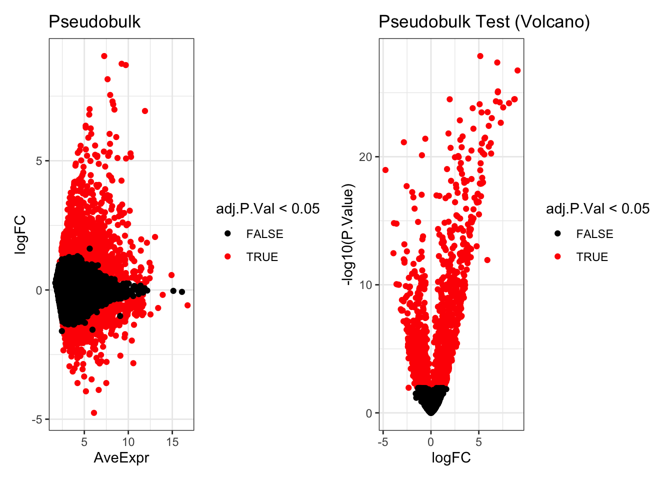
de_result_pseudobulk <- arrange(de_result_pseudobulk , adj.P.Val)Look at the significantly differentially expressed genes:
head(de_result_pseudobulk)
#>           logFC   AveExpr        t      P.Value
#> ISG20  5.151090 10.311187 34.62460 1.377577e-28
#> ISG15  6.926462 11.895928 33.45672 4.402969e-28
#> CXCL11 9.051653  7.260525 32.07090 1.838679e-27
#> IFIT3  6.980913  8.420719 28.54319 9.234346e-26
#> HERC5  6.998957  5.602349 28.68162 7.853707e-26
#> TMSB10 1.959063 11.466981 27.48469 3.264041e-25
#>           adj.P.Val        B
#> ISG20  9.940598e-25 55.27733
#> ISG15  1.588591e-24 54.12183
#> CXCL11 4.422636e-24 51.56638
#> IFIT3  1.332701e-22 48.32088
#> HERC5  1.332701e-22 48.02111
#> TMSB10 2.950103e-22 47.34483
p1 <- ggplot(de_result_pseudobulk, aes(x=AveExpr, y=logFC, col=adj.P.Val < 0.05)) +
  geom_point() +
  scale_colour_manual(values=c('TRUE'="red",'FALSE'="black")) +
  theme_bw() +
  ggtitle("Pseudobulk")


p2 <- ggplot(de_result_pseudobulk, aes(x=logFC, y=-log10(P.Value), col=adj.P.Val < 0.05)) +
  geom_point() +
  scale_colour_manual(values=c('TRUE'="red",'FALSE'="black")) +
  theme_bw() +
  ggtitle("Pseudobulk Test (Volcano)")

p1 + p2