10 Batch Correction
10.1 Do we need batch correction?
There are regions in the UMAP where we can see some separation by sample. This is common in spatial data, especially when working with human data.
(In fact, this example isn’t too bad, but for the purposes of this work, we will go through the process of batch correction).
DimPlot(so, group.by='tissue_sample')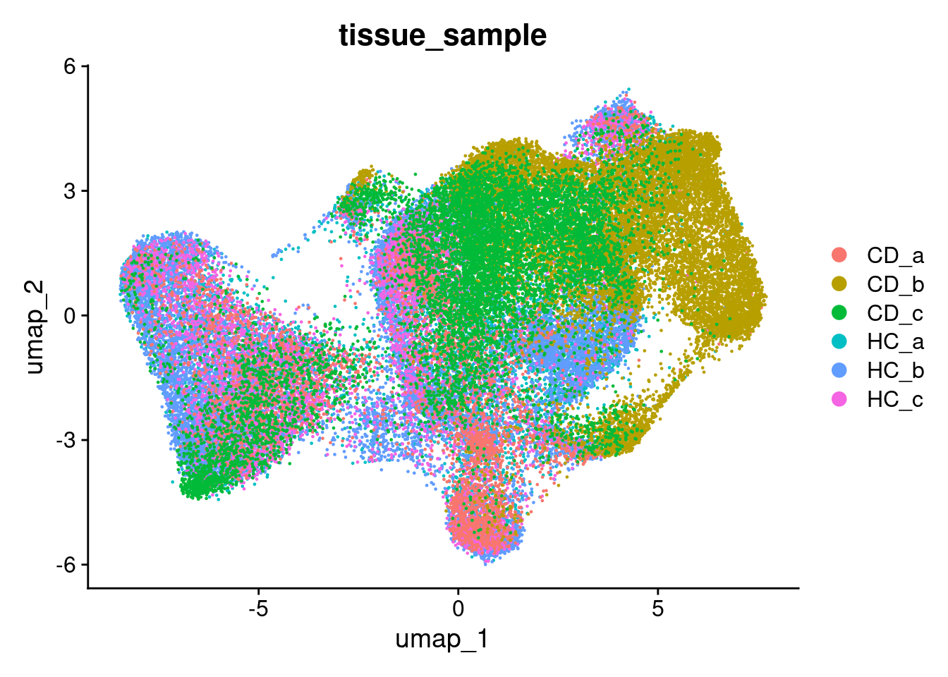
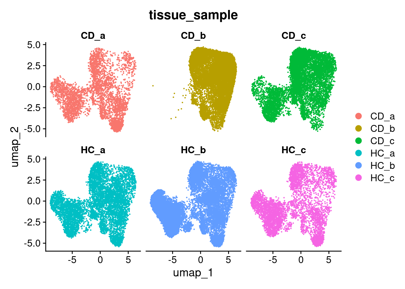
This becomes more obvious if we split the plot by sample as well;
DimPlot(so, group.by='tissue_sample', split.by = 'tissue_sample', ncol = 3)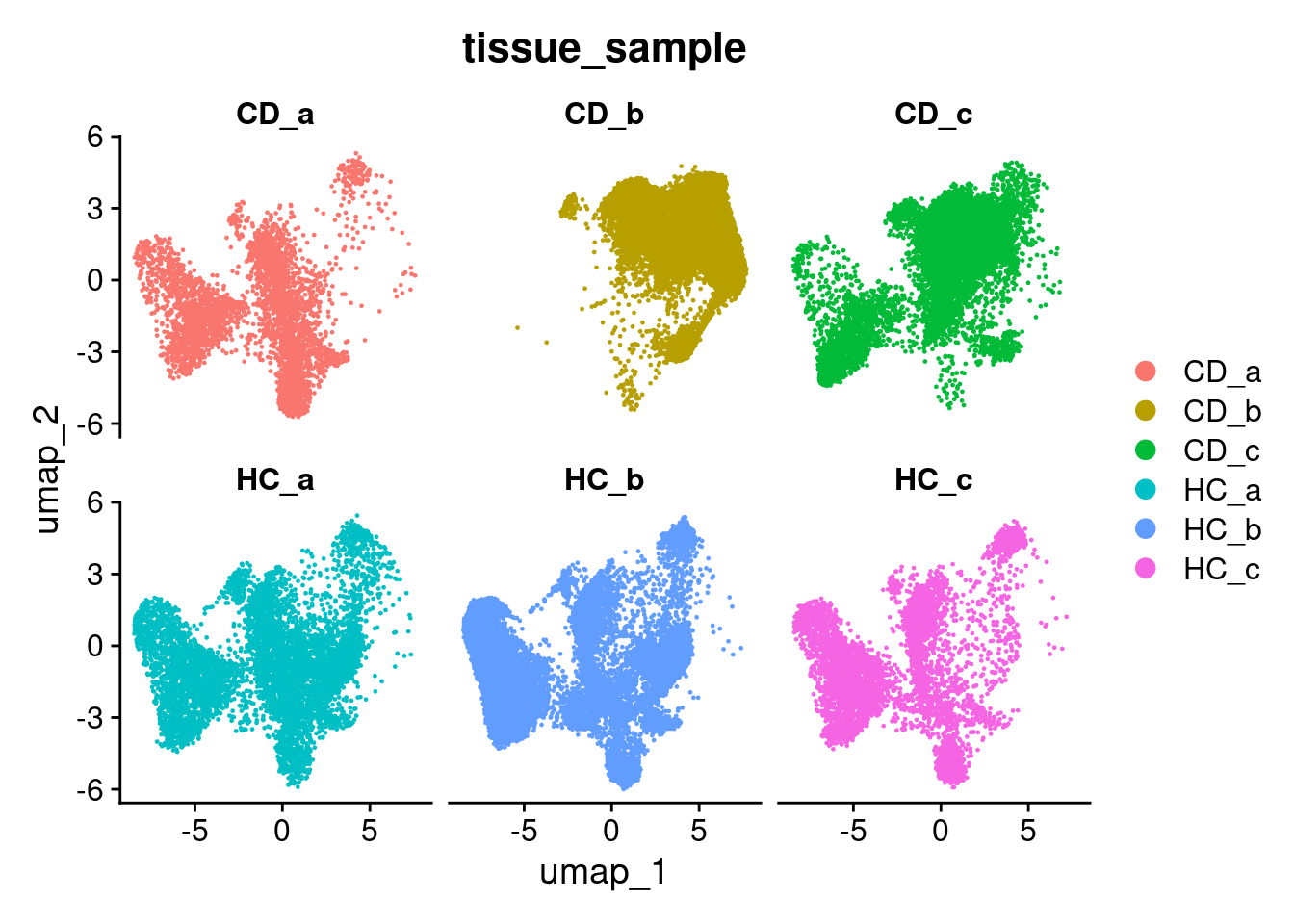
If were were to continue on to cell clustering at analysis at this point, we might find that we build clusters around individual samples. We instead want to make cell clusters that form around cell ‘types’ (or transcriptionallly similar cell states) across multiple samples, which can be matched and compared across experimental groups.
10.2 Running batch correction
We can apply a batch correction or integration method to adjust our principal components to deemphasise the betweeen-sample effect. Seurat implements several such methods, and has a full ‘Introduction to scRNA-seq integration’ vignette. We will use the ‘harmony’ method, from Korsunsky et al 2019: https://www.nature.com/articles/s41592-019-0619-0
Its worth noting that these same methods can be applied to combine data from multiple experiments (e.g. public data), or even technologies!
This is one of the most computationally intensive steps of the analysis. It can take hours to run and use many Gb of RAM, scaling with the size of your experiment.
This is the code to the integration and generate a new UMAP. Do not run this code today!
  # https://satijalab.org/seurat/articles/seurat5_integration
  # Slow?
  so <- IntegrateLayers(so, method = HarmonyIntegration, orig.reduction = "pca", new.reduction = "harmony")
  so <- RunUMAP(so, dims=1:num_dims, reduction = 'harmony')

  DimPlot(so, group.by='tissue_sample')


  ## TODO Remove clustering from this section, update object
  #so <- FindNeighbors(so, reduction = "harmony", dims = 1:num_dims)
  #so <- FindClusters(so, resolution = 0.2)
  # don't talk about optimisation of clusters, point people at single cell resources.
}
Instead, load up a version of the object with theis data.
seurat_file_01_preprocessed_subset <- here("data", "GSE234713_CosMx_IBD_seurat_01_preprocessed_subsampled.RDS")
so <- readRDS(seurat_file_01_preprocessed_subset)
Looking in the summary of the seurat object we see 3x dimensional reductions:
- pca : Our original principal components, with no batch correction.
- harmony : The harmony output, values like the PCA, but adjusted for batch correction.
- umap : Our new umap which was based on harmony (because we passed reduction = ‘harmony’ to RunUMAP). This overwrote the old UMAP.
so## An object of class Seurat
## 999 features across 50662 samples within 2 assays
## Active assay: RNA (980 features, 200 variable features)
## 13 layers present: counts.GSM7473682_HC_a, counts.GSM7473683_HC_b, counts.GSM7473684_HC_c, counts.GSM7473688_CD_a, counts.GSM7473689_CD_b, counts.GSM7473690_CD_c, data.GSM7473682_HC_a, data.GSM7473683_HC_b, data.GSM7473684_HC_c, data.GSM7473688_CD_a, data.GSM7473689_CD_b, data.GSM7473690_CD_c, scale.data
## 1 other assay present: negprobes
## 3 dimensional reductions calculated: pca, harmony, umap
## 6 spatial fields of view present: GSM7473682_HC_a GSM7473683_HC_b GSM7473684_HC_c GSM7473688_CD_a GSM7473689_CD_b GSM7473690_CD_cWhen plotting the new UMAP, the samples are move overlayed. This will make for better vizualisation.
DimPlot(so, group.by='orig.ident')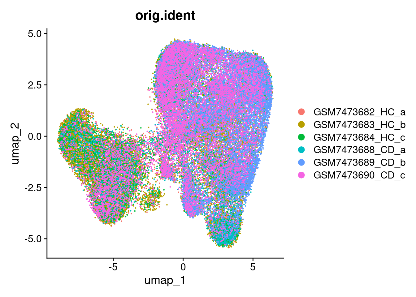
DimPlot(so, group.by='tissue_sample', split.by = 'tissue_sample', ncol = 3)